Pan-Antarctic evaluation of National Snow and Ice Data Center (NSIDC) sea ice drift product using high-resolution SAR and buoy data

The recent historic minima in Antarctic sea ice extent suggest the possibility of new thermodynamic and dynamic conditions across the Southern Ocean. In investigating these thermodynamic and dynamic sea ice behaviors, it is essential to observe sea ice drift with high quality. However, while the relatively abundant and reliable buoy data in the Arctic guarantees a robust Arctic sea ice drift observation, the Antarctic sea ice drift product merely relies on passive microwave (PMW) data due to the lack of pan-Antarctic drifting buoy data. In this study, we assess the uncertainty of the Antarctic sea ice drift product from 2015 to 2023 by using drifting buoys in the Weddell Sea and synthetic aperture radar (SAR) sea ice drift across the Southern Ocean. The comparison between PMW and buoy ice drift shows that PMW-derived sea ice drift tends to underestimate drift speed by 2–3 km d⁻¹, particularly under low ice concentration conditions, while drift direction agrees well with a marginal bias. Based on the accurate high-resolution sea ice drift estimation from SAR imagery (−6° of angle difference and 0.1 km d⁻¹ of speed difference with buoy ice drift), we assess the pan-Antarctic uncertainties of PMW sea ice drift. We found a widespread ∼ 1 km d⁻¹ underestimation of ice drift speed across the Southern Ocean, particularly in the east Weddell Sea and west Ross Sea. Ice drift direction generally shows negligible bias across the Southern Ocean, but the east Weddell Sea shows 10–20° of clockwise bias. Such a wide underestimation is attributed to the optimal interpolation that smooths ice velocity and raises uncertainties around the marginal ice zone. Based on this understanding of PMW-derived Antarctic sea ice drift estimation, it is important to improve the sea ice velocity estimation in the Southern Ocean.

1 Introduction

Antarctic sea ice has recently recorded historic minima and a record-low maximum extent over the last few years, a decline potentially driven by complex and interacting climatological factors, such as warming ocean temperatures and atmospheric circulation changes (Raphael and Handcock, 2022; Turner et al., 2022; Purich and Doddridge, 2023; Wang et al., 2024). Given that Antarctic sea ice largely exists in an open-ocean environment and is thus highly dependent on wind from the continent (Kimura, 2004; Holland and Kwok, 2012; Kwok et al., 2017), the study of sea ice dynamics is critical for understanding the future state of the Antarctic sea ice cover under recent climate change. To monitor Antarctic sea ice drift on a large scale, passive microwave (PMW) data have been commonly employed. PMW observations offer significant advantages due to their wide spatial coverage, which facilitates the investigation of large-scale drift patterns across the entire Southern Ocean (Kwok et al., 2017). Additionally, the availability of long-term data records spanning more than four decades since 1979 through a combination of various PMW sensors, such as Scanning Multichannel Microwave Radiometer (SMMR), Special Sensor Microwave/Imager (SSM/I), Special Sensor Microwave Imager/Sounder (SSMIS), and Advanced Microwave Scanning Radiometer (AMSR), have allowed comprehensive exploration of long-term sea ice velocity trends (Heil et al., 2006; Kwok et al., 2017).

However, while PMW-derived sea ice drift is valuable for characterizing extensive spatial patterns and long-term trends, it is inherently subject to significant uncertainties (on the scale of several kilometers) due to its coarse spatial resolution (Kimura, 2004; Kwok et al., 2017). To mitigate the uncertainties associated with PMW-alone sea ice drift extraction, various supplementary data, including drifting buoys and atmospheric reanalysis, have been integrated with PMW observations (Tschudi et al., 2019). Then, the generation of daily sea ice motion products across the polar oceans typically employs an optimal interpolation scheme, where different weight values are assigned to each motion estimate based on the data source and distance from the grid point. Among various data sources, buoy data are considered most accurate and thus assigned the highest weights (Tschudi et al., 2019). In the Arctic, this optimal interpolation approach enables a relatively accurate estimation of sea ice velocity owing largely to the frequent availability of buoy data across the Arctic Ocean. In the Antarctic, the quality of sea ice drift products remains more uncertain due to the sparsity of drifting buoy data across the Southern Ocean (Tschudi et al., 2020). Although several buoys have been deployed in the Southern Ocean, most are concentrated near the Weddell Sea, thereby limiting the representativeness of these data across the entire Southern Ocean. Furthermore, since Antarctic sea ice typically exhibits higher daily displacement and deformation rates than the Arctic, identifying the spatial coherence of PMW-derived brightness temperature features can be challenging during feature tracking and matching (Kwok, 2010; Kwok et al., 2017; Heil et al., 2001).

Consequently, it is crucial to quantify and understand the uncertainty of PMW-derived sea ice drift and explore opportunities for improving this estimation. In general, drifting buoys have served as the most common and direct method for validating PMW-derived sea ice drift. However, although PMW-derived sea ice drift products have been widely validated against buoys across the Arctic Ocean (Kwok et al., 1998; Lavergne et al., 2010; Rozman et al., 2011; Hwang, 2013; Gui et al., 2020), a comparable large-scale validation over the Southern Ocean has been hindered by the limited deployment of buoys. For example, Kwok et al. (1998) reported that PMW-derived sea ice drift had errors of 0.6±7.4 and 0.1±8.2 km d⁻¹ in horizontal and vertical velocity components, respectively, on a polar stereographic map projection, achieving a correlation coefficient of 0.67 when compared with buoy data. However, their assessment was constrained to a single year (1992) and focused exclusively on the Weddell Sea. Similarly, Schwegmann et al. (2011) conducted a long-term assessment of PMW-derived sea ice drift using buoy data from 1989 to 2005, and they found that the PMW sea ice drift product exhibited errors of 1.04±7.86 and 0.86±7.86 km d⁻¹ in horizontal and vertical velocity components, respectively, with a correlation coefficient of ∼ 0.6. Tian et al. (2022) validated a PMW-derived sea ice drift product, specifically daily sea ice motion vectors derived from ascending, descending, and combined tracks, using buoy observations in the Weddell Sea and Ross Sea. The PMW sea ice drift products from the Ocean and Sea Ice Satellite Application Facility (OSI SAF) have also been validated against buoy data in the Southern Ocean (Lavergne and Down, 2022, 2024). However, these buoy-based assessments are confined to a limited period and geographic extent, restricting their ability to capture the full spatiotemporal variability of uncertainties across the Southern Ocean.

Moving beyond the limited buoy coverage of the Weddell Sea, high-resolution synthetic aperture radar (SAR) imagery has been leveraged to validate PMW sea ice drift in regions where drifting buoy data are sparse or absent. Kwok (2005) utilized RADARSAT SAR imagery (with a resolution of ∼ 150 m) to validate PMW sea ice drift in the Ross Sea in 1998 and 2000. According to their comparison results, PMW sea ice drift exhibited a correlation coefficient ranging from 0.77 to 0.88 and a mean difference between −0.4 and 0.4 km d⁻¹, demonstrating a consistency in the quality of PMW-derived sea ice motion across both the Fram Strait and Ross Sea. Furthermore, Kwok et al. (2017) used Envisat SAR imagery for the pan-Antarctic validation of PMW-derived sea ice drift from 2007 to 2010. This validation showed a correlation coefficient of 0.73–0.86 and a mean difference of −0.5 to 1.5 km d⁻¹ between PMW and SAR ice drift products. Although these previous studies demonstrated the effectiveness of PMW-derived sea ice drift for understanding synoptic and longer-term drift patterns across the Southern Ocean (Kwok et al., 2017), it is still necessary to further validate PMW sea ice drift and understand its uncertainty sources in the context of the emerging new state of Antarctic sea ice (Purich and Doddridge, 2023).

In this study, we aim to validate PMW-derived Antarctic sea ice drift using high-resolution Sentinel-1 SAR imagery. Since 2014, Sentinel-1 SAR has provided near-global coverage of the polar oceans with frequent revisit periods, often less than 2–3 d (Torres et al., 2012). Furthermore, the accessibility of Sentinel-1 data through the Google Earth Engine (GEE) cloud-based platform has facilitated its widespread use for accurate tracking of mobile features in the polar environment, including sea ice and icebergs (Muckenhuber et al., 2016; Korosov and Rampal, 2017; Muckenhuber and Sandven, 2017; Koo et al., 2021; Howell et al., 2022; Koo et al., 2023). We first perform a quality assessment of the Sentinel-1 SAR-based sea ice feature tracking algorithm for the Antarctic, using high-accuracy drifting buoy data where available. Following this initial assessment of Sentinel-1 sea ice drift, the SAR-derived sea ice drift is established as a reliable high-resolution reference for validating the PMW sea ice drift product. By leveraging the extensive 9-year Sentinel-1 data and cloud-friendly processing via GEE, we investigate the spatiotemporal variability of errors inherent in PMW-derived sea ice drift. Ultimately, our comprehensive quality assessment seeks to identify the key limitations of current PMW-derived sea ice velocity products and propose strategies for their future improvement.

2 Data and Methods

2.1 Passive microwave sea ice drift

In this study, we use the Polar Pathfinder Daily 25km EASE-Grid Sea Ice Motion Vectors product (version 4) archived and distributed by the NASA Snow and Ice Distributed Active Archive Center (DAAC) at the National Snow and Ice Data Center (NSIDC) (Tschudi et al., 2019, 2020). Although this product employs optimal interpolation to combine three independent data sources in the Arctic – (i) gridded PMW satellite imagery, (ii) winds from reanalysis fields, and (iii) drifting buoy positions – the Antarctic sea ice motion is derived solely from gridded and optimally interpolated PMW satellite imagery. To generate gridded sea ice drift, this product first computes daily-averaged PMW brightness temperatures on the EASE grid. Then, it uses a feature-tracking algorithm that calculates cross-correlations between spatial patterns on different days, i.e., the maximum cross-correlation (MCC) pattern-matching method (Emery et al., 1991, 1995; Tschudi et al., 2020). This method involves selecting two spatially coincident and temporally consecutive satellite images, defining a search window around a grid cell, and translating the latter image relative to the earlier one within this window. Then, the spatial offset corresponding to the maximum correlation value is taken as the most probable ice displacement. This offset is converted to ice velocity by dividing the spatial displacement by the time separation between the two images. For the study period (2015–2023), 37H GHz, 37V GHz, 91H GHz, and 91V GHz channels of the Special Sensor Microwave/Imager and Sounder (SSMIS) were used as the PMW imagery sources (Tschudi et al., 2019). However, since the intrinsic PMW sensor footprint is coarse, the resultant sea ice motion field is coarse and noisy. To address this limitation and achieve sub-pixel resolution, the MCC method used for this product incorporates 4 × oversampling, which improves the effective SSMIS sampling interval to 6.25 km d⁻¹.

To generate the daily gridded Antarctic sea ice motion fields, the PMW-based sea ice motion is optimally interpolated (i.e., kriging). In this kriging interpolation, the sea ice motion vector (comprising the u and v velocity components) at a given grid cell is calculated by assigning weights to nearby available sea ice velocity values, and those weighted velocities are averaged to estimate the grid cell value. This weighting factor (w) is inversely dependent on the distance (d) from the source data point, determined by the following exponential function:

$$\begin{array}{}\text{(1)}& w=C{e}^{-d/D}\end{array}$$

where D represents the length scale constant, empirically determined to be 417 km (Tschudi et al., 2020), and C is the source-based coefficient (0.8 for SSMIS-based sea ice motion; for the Arctic product, this coefficient is 0.95 for buoy data and 0.45 for wind). The optimal interpolation effectively transforms the sparse and/or noisy individual motion estimates into a smoothly varying combined daily motion grid. It is important to acknowledge that optimal interpolation relies on the ideal assumptions of stationarity, homogeneity, and isotropy in the data field, which are often violated in real-world sea ice dynamics. We refer to Tschudi et al. (2019, 2020) for a detailed description of this sea ice motion product.

2.2 Sentinel-1 SAR sea ice drift

In this study, we acquire Sentinel-1 SAR images covering the entire Southern Ocean over a 9-year period, from 2015 to 2023. The Sentinel-1 mission consists of two identical satellites, Sentinel-1A (launched in April 2014) and Sentinel-1B (launched in April 2016; operations ended in December 2021). The combined constellation provides a 6 d revisit cycle based on a 12 d revisit cycle for each satellite. Sentinel-1 satellites carry a single C-band SAR with a center frequency of 5.405 GHz and a wavelength of 5.6 cm. We utilize the Level-1 HH polarization band images in Extra Wide Swath (EW) mode from the Ground Range Detected (GRD) scenes, which have a resolution of 40 m. We access and process these images via GEE (Gorelick et al., 2017), where each scene is pre-processed using the Sentinel-1 Toolbox, which includes (i) thermal noise removal, (ii) radiometric calibration, and (iii) terrain correction (orthorectification) (https://developers.google.com/earth-engine/guides/sentinel1, last access: 16 September 2026).

We divide the entire Southern Ocean into multiple 250 km × 250 km super-grids on the EASE projection and collect all available Sentinel-1 images for each super-grid via GEE. For Sentinel-1 images covering more than 30 % of a super-grid cell, we downscale the original ∼ 40 m resolution images to 120 m resolution on the EASE projection. This downscaling is performed to export the images as the same-dimension arrays into a Python environment using the geemap package (Wu, 2020). This downscaling also serves two purposes: reducing speckle noise in SAR backscatter imagery and reducing the computational load required for processing a large number of images. Additionally, to ensure a reliable estimation of sea ice drift, we only use Sentinel-1 image pairs with a temporal separation of less than 4 d (96 h).

For all collected Sentinel-1 image pairs within each super-grid, we retrieve sea ice drift using the motion retrieval algorithm developed by Nansen Environmental and Remote Sensing Center (NERSC) (Korosov and Rampal, 2017; Muckenhuber and Sandven, 2017). This algorithm achieves high accuracy (reported positional error below 300 m) and computational efficiency (processing time of less than one minute per Sentinel-1 image pair) by combining feature tracking and pattern matching methods (Korosov and Rampal, 2017; Muckenhuber and Sandven, 2017; Park et al., 2021). The initial feature-tracking algorithm, called ORB (Oriented FAST and Rotated BRIEF), is adopted and tuned for retrieving a first-guess sea ice drift from the Sentinel-1 SAR images. Then, the next pattern-matching algorithm, based on MCC calculation, is used further to derive sea ice drift on a regular grid. First, feature tracking automatically identifies keypoints in a pair of Sentinel-1 SAR images as a vector of 256 binary descriptors (Lowe, 2004); the number of keypoints is set to 20 000 based on empirical experiments. For each keypoint on the first image, a ratio between the smallest and the second smallest Hamming distance (number of the descriptors in the vector with different values; Hamming, 1950) to the keypoints on the second image is computed. If the ratio is below a threshold (set to 0.7 in this study), the keypoint with the smallest Hamming distance is considered matched. If this ice displacement exceeds 40 km d⁻¹, this vector is omitted as incorrect (Muckenhuber et al., 2016; Korosov and Rampal, 2017). Since these keypoints are heterogeneously distributed in space, the feature-tracking results are approximated on a regular grid using linear interpolation.

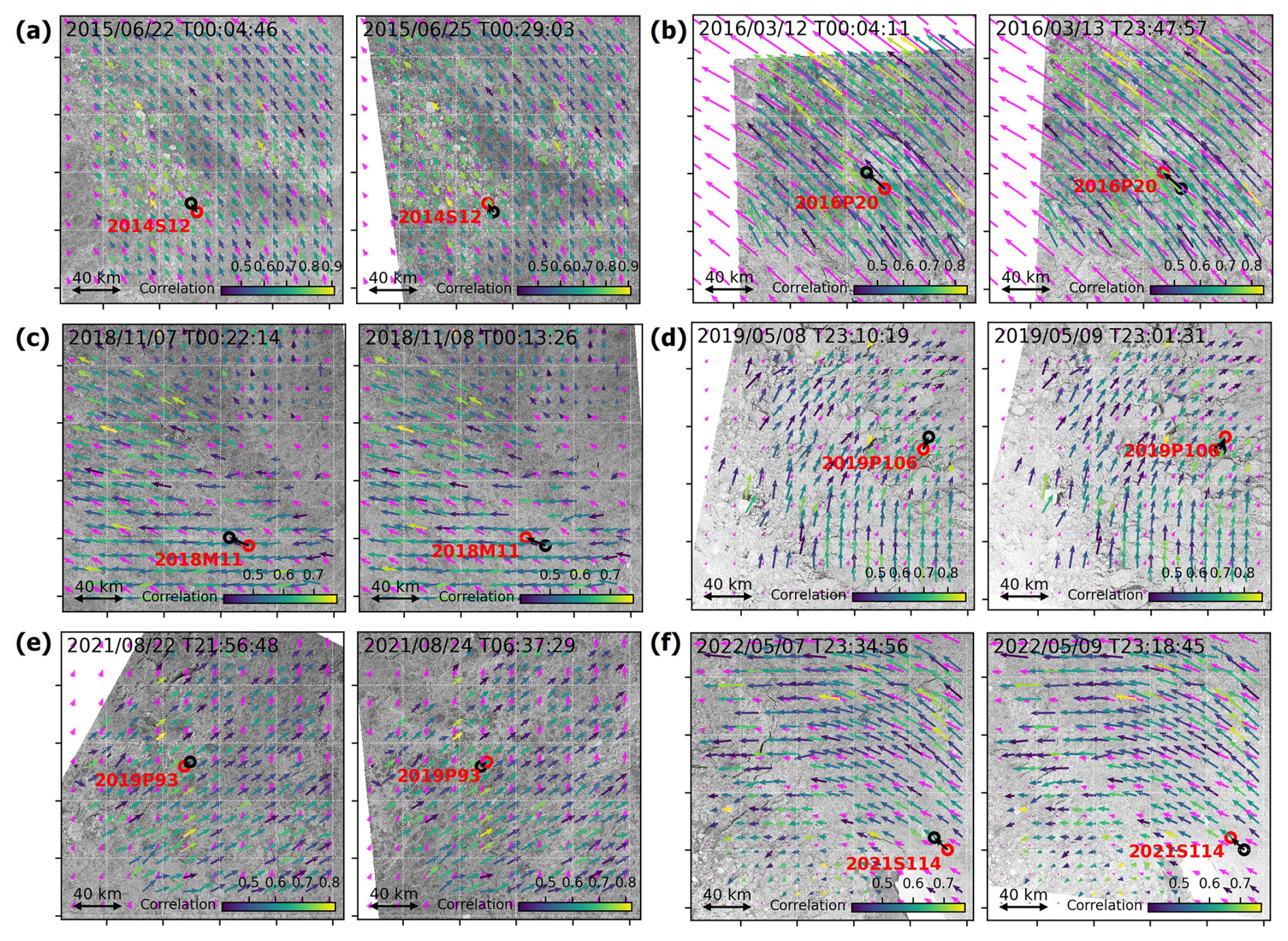
Figure 1 Derivation of sea ice drift from SAR images nearby (a) buoy 2014S12 from 22 to 25 June 2015, (b) buoy 2016P20 from 12 to 13 March 2016, (c) buoy 2018M11 from 7 to 8 November 2018, (d) buoy 2019P106 from 8 to 9 May 2019, (e) buoy 2019P93 from 22 to 24 August 2021, and (f) buoy 2021S114 from 7 to 9 May 2022. Colored arrows indicate SAR-derived sea ice drift, with colors representing the correlation of feature tracking (see bottom-right color bar). Magenta arrows indicate PMW sea ice drift, and black arrows indicate the movements of buoys between the SAR acquisition times; red circles denote the location of the buoy at each image, and buoy IDs are annotated in red. The lengths of the vectors correspond to the actual sea ice displacement.

Next, this approximated ice drift on a regular grid serves as the first guess for the subsequent, more precise pattern-matching method. A template t is defined around a point of interest in the first image, and the corresponding x and y coordinates in the second image are estimated based on the initial feature-tracking ice drift approximation. A larger sub-image s is then extracted from the second image, centered at these coordinates. Then, the template t is rotated within a range of angles (rotated template t_ROT), and the rotation angle that provides the maximum cross-correlation between the rotated template t_ROT and s within a searching range D is determined. After the optimal rotation angle between two image scenes is found, the position of the maximum cross-correlation (r_MAX) is identified as the resultant positional offset from the first image to the second image. If this maximum cross-correlation r_MAX falls below a threshold of 0.4, we disregard this drift vector as unreliable. Based on the results from Korosov and Rampal (2017) and our trial-and-error experiments, we set the template size (T) to 20 pixels and the searching range D to 35 pixels. A template size of 20 pixels results in a nominal SAR sea ice drift resolution of approximately 2.4 km (120 m downsampled SAR resolution × 20 pixels). As illustrated in Fig. 1, the resultant SAR-derived sea ice drifts appear reliable and show good agreement with buoy sea ice drift (Fig. 1). More details about this SAR-based ice drift retrieval algorithm are described in Korosov and Rampal (2017), and the open source software of this algorithm is publicly available (https://github.com/nansencenter/sea_ice_drift, last access: 16 September 2026).

2.3 Antarctic buoys

For the comprehensive validation of PMW and SAR sea ice drift, we utilize position data from drifting buoys deployed across the Southern Ocean as part of the International Programme for Antarctic Buoys (IPAB). These buoys record precise latitude and longitude positions every 1–3 h, providing accurate and precise sea ice drift information. We found 99 available drifting buoys spanning from 2015 to 2023, with the majority concentrated in the Weddell Sea region (Fig. 2). Buoys deployed in the Weddell Sea typically follow the clockwise circulation of the Weddell Gyre (Fig. 2). However, upon exiting the Weddell Sea, these buoys are often transported by the Antarctic Circumpolar Current, moving outside the primary sea ice boundary. To ensure that buoy motion accurately represents sea ice drift, we exclude any buoy data points where the coincident sea ice concentration is below 15 %. Although some buoys are available in the Ross Sea near the McMurdo Sound, their limited distribution prevents them from fully representing regional sea ice drift. We calculate the velocity vectors from the recorded buoy position changes to serve as the reference sea ice drift, which is then compared with coincident PMW and SAR drift observations.

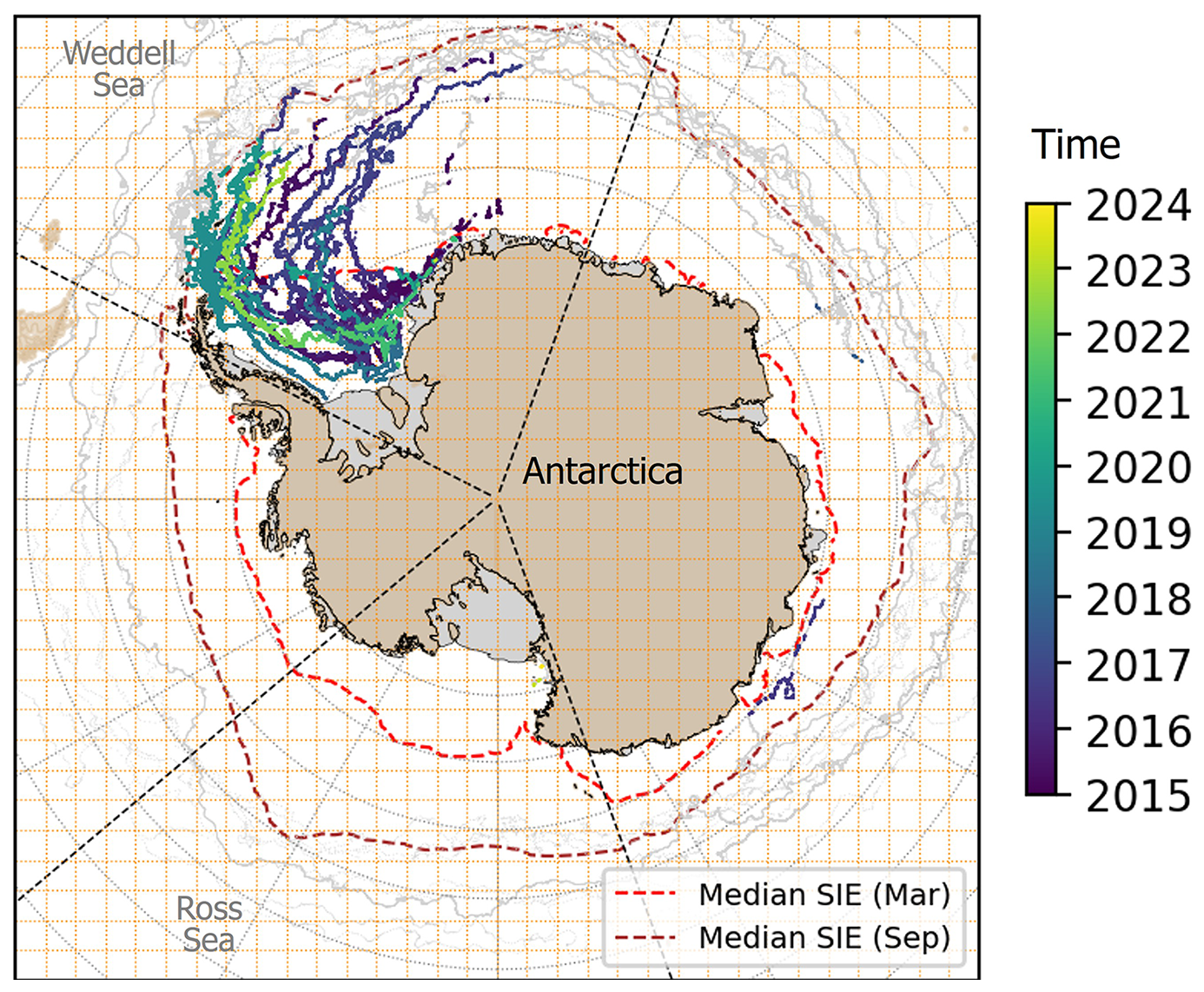
Figure 2 Distribution of Antarctic drifting buoys from 2015 to 2023. The buoys inside sea ice cover (SIC > 15 %) are colorized by the times of the buoy locations, whereas the buoys outside sea ice cover are displayed in gray points. The red dashed line indicates the median March sea ice extent (SIE) in 1981–2010, and the brown dashed line indicates the median September SIE in 1981–2010. While most of the buoys are deployed in the Weddell Sea, these buoys rarely pass through the sea ice area in other regions. Orange dashed lines show the 250 km × 250 km super-grid for Sentinel-1 data collection.

2.4 Spatial and temporal sampling for data comparison

It is essential to note that the PMW, SAR, and buoy sea ice drift observations possess distinct spatial and temporal scales. Therefore, we employ three different spatiotemporal sampling schemes to facilitate robust comparisons: (i) SAR-buoy, (ii) PMW-buoy, and (iii) PMW-SAR.

SAR-buoy comparison: Sentinel-1 SAR provides gridded sea ice drifts between two image acquisition times, whereas buoys provide regular point-to-point track movement every 1–3 h. To match these data, we first extract the buoy displacement vector over the exact time interval between two SAR image scenes. The resulting x and y displacements, divided by the time difference, constitute the buoy-derived sea ice drift velocity. For the corresponding SAR sea ice drift, we calculate the mean of SAR vectors located within a 25 km radius of the buoy location. Following the recommendation of Korosov and Rampal (2017) to ensure reliable drift estimates, this comparison is restricted to areas where the sea ice concentration was greater than 85 %.

PMW-buoy comparison: The PMW product provides daily 25 km gridded sea ice drifts, which must be reconciled with the hourly (or 3-hourly) buoy track movements. To achieve temporal consistency, we first calculate the daily displacement of the buoys. This daily buoy displacement is then compared with the mean of the PMW sea ice drift vectors located within a 25 km radius of the buoy's central location. Unlike the SAR-buoy comparison, this PMW-buoy comparison is conducted across the entire available product area, where the sea ice concentration is greater than 15 % (Tschudi et al., 2019). We note that both SAR and PMW ice drift vectors represent the average ice drift within a large area of radius 25 km, whereas the buoy vectors represent point-like ice drift at deployed ice floes. This scale mismatch, alongside spatial and temporal collocation errors, introduces a representativeness error that may partly explain the observed discrepancies between satellite-derived and buoy-measured ice drift (Sumata et al., 2014; Lavergne et al., 2010). Since this representativeness error is difficult to fully separate from intrinsic retrieval errors, the validation statistics reported in this study likely contain contributions from both error sources.

PMW-SAR comparison: Although both PMW and SAR provide large-scale sea ice drift fields, the PMW product has coarse spatial resolution (25 km) and a regular daily record, while the SAR product has a finer spatial resolution (∼ 2.4 km) and irregular sampling time (between image acquisitions). For each 25 km PMW grid cell, we calculate the mean SAR-derived sea ice drift if there are more than 10 available SAR vectors within a 25 km radius of the PMW cell center. We also calculate the average PMW-derived sea ice displacement at that PMW cell between the Sentinel-1 image acquisition times using the daily PMW sea ice drift. Consequently, we compare SAR-derived and PMW-derived sea ice drifts between SAR acquisition times for 25 km PMW grid cells. Given the requirement for high-quality SAR drift input, this comparison is also limited to regions with sea ice concentration greater than 85 %. We also note that we present the results only from March to November due to low sea ice cover in the summer months (December to February).

Validation metrics: To quantify the accuracy of sea ice drift estimates from each comparison scheme, we compute two primary vector metrics between ice drift vectors: (1) angle difference and (2) speed difference. Additionally, for the direct comparisons against the buoy reference data (SAR-buoy and PMW-buoy comparisons), we also calculate the root mean square errors (RMSEs), mean difference (MD), and correlation coefficient (R) between u and v component vectors. We note that these u and v vector components are the horizontal and vertical components on the EASE grid, not the typical zonal and meridional components.

3 Results

We assess the PMW-derived sea ice drift using two independent reference datasets: drifting buoys and SAR-derived sea ice drift. Before using the SAR-derived sea ice drift as a high-resolution reference dataset for PMW validation, we first quantify its accuracy using the available buoy data.

3.1 Comparison between SAR-derived and buoy ice velocities

Figure 3 presents the comparison between SAR and buoy sea ice drift. The SAR ice drift demonstrates an RMSE of 2.0 km d⁻¹ and R of 0.92 in u velocity component and an RMSE of 3.3 km d⁻¹ and R of 0.85 in v velocity component (Fig. 3a and b). The MDs of the u and v components between SAR and buoy velocities (ε_u and ε_v) are $-\mathrm{0.1}\pm \mathrm{2.0}$ and $-\mathrm{0.1}\pm \mathrm{3.2}$ km d⁻¹, respectively, which indicates minimal biases in SAR-derived ice drift compared to the buoys (Fig. 3c). Furthermore, the angle difference ($-\mathrm{5.9}\pm \mathrm{38.6}$°) and speed difference (0.1±2.9 km d⁻¹) between SAR and buoy vectors are close to zero. These results confirm that SAR imagery is an effective and accurate tool for deriving sea ice drift where buoy measurements are unavailable in the Southern Ocean (Fig. 3d and e). Spatially, there are no significant patterns observed in the errors of the SAR ice velocity (Fig. 3f and g), although the available SAR-buoy comparison pairs are predominantly located in the Weddell Sea.

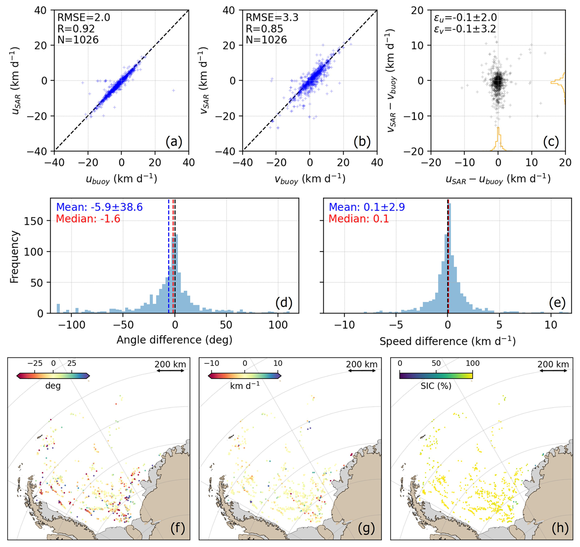
Figure 3 (a) Scatter plot between u-component sea ice drift from buoys and SAR imagery, (b) scatter plot between v-component sea ice drift from buoys and SAR imagery. We note that these u and v components represent the orthogonal (horizontal and vertical) components on the Equal-Area Scalable Earth (EASE) Grid projection, not the zonal and meridional drift. (c) Error distribution of the u and v sea ice drift components. Distribution of (d) angle difference and (e) speed difference between SAR and buoy sea ice velocities. Location of buoys visualized by (f) angle difference, (g) speed difference, and (h) sea ice concentration. We note that SAR-buoy pairs were available only in the Weddell Sea.

3.2 Comparison between PMW and buoy ice velocities

Figure 4 illustrates the comparison results between PMW and buoy sea ice drift. As expected, the PMW sea ice drift exhibits relatively larger errors compared to the SAR sea ice drift product discussed previously. The PMW ice drift yields an RMSE of 7.1 km d⁻¹ for u velocity component and 7.9 km d⁻¹ for v velocity component (Fig. 4a and b). These error magnitudes are significantly greater than the RMSE of 2.90–2.93 km d⁻¹ reported for the Arctic (Tschudi et al., 2019). The larger RMSE in the Antarctic is primarily attributed to the omission of buoy data in the optimal interpolation scheme used for the Antarctic sea ice drift product. Nevertheless, the MDs of the u and v components (ε_u and ε_v) are found to be 0.2±7.1 and $-\mathrm{0.6}\pm \mathrm{7.8}$ km d⁻¹, respectively (Fig. 3c). These low mean bias values are consistent with those reported for the Arctic product and prior Antarctic validation studies (Kwok et al., 1998; Tschudi et al., 2019; Schwegmann et al., 2011). Analysis of the vector metrics indicates that the PMW sea ice drift is negligibly biased in direction (3–4° angle difference) and consistently underestimates the sea ice speed by an average of 2–3 km d⁻¹ (Fig. 4d and e).

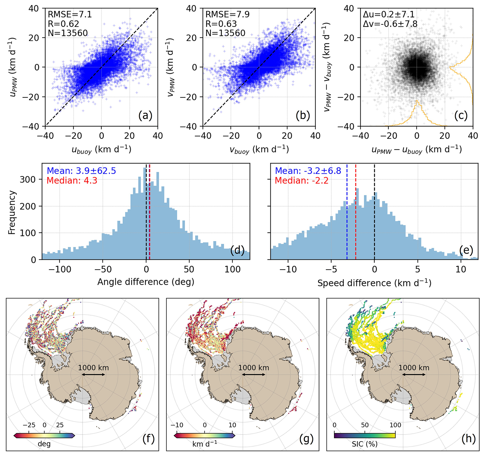
Figure 4 (a) Scatter plot between u-component sea ice drift from buoys and PMW, (b) scatter plot between v-component sea ice drift from buoys and PMW. (c) Error distribution of the u and v sea ice drift components. (d) Distribution of angle difference and (e) speed difference between PMW and buoy sea ice velocities. Location of buoys visualized by (f) angle difference, (g) speed difference, and (h) sea ice concentration.

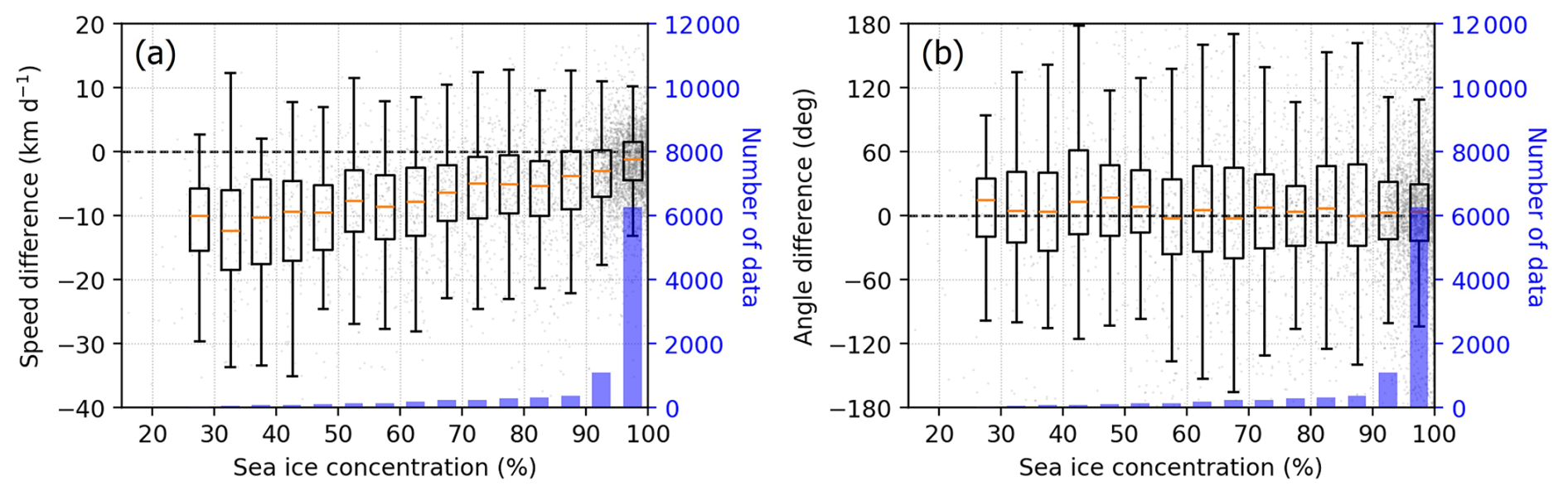
Figure 5 (a) Speed difference between PMW and buoy sea ice drift by sea ice concentration. (b) Angle difference between PMW and buoy sea ice drift by sea ice concentration.

An interesting and conspicuous finding is the strong dependence of the PMW sea ice drift underestimation on sea ice concentration (SIC) (Figs. 4h and 5a). In regions with high SIC (95 %–100 %), which comprise approximately 64 % of the total comparison data, the PMW sea ice velocity exhibits an underestimation (negative bias) of only ∼ 1.52 km d⁻¹. For SIC > 85 %, the negative bias is ∼ 1.97 km d⁻¹. However, this negative speed bias increases substantially as SIC decreases, reaching an underestimation of ∼ 11.47 km d⁻¹ on average in areas with SIC below 50 % (Fig. 5a). In contrast, the angle difference shows no significant trend or dependence on SIC (Fig. 5b). This finding suggests two potential hypotheses: (i) the PMW-based feature tracking method inherently yields lower accuracy under low SIC conditions; and (ii) the optimal interpolation scheme used in the product introduces a systemic underestimation of sea ice speed, particularly near the sea ice edge. We will discuss the potential impact of interpolation and sea ice edge dynamics in detail in Sect. 4.

3.3 Comparison between PMW-derived and SAR-derived ice velocities

The SAR-buoy sea ice drift comparison in Sect. 3.1 established the high accuracy of the SAR product, confirming its suitability as a reliable, high-resolution reference for sea ice drift. By using this SAR-derived sea ice drift, we extend the uncertainty assessment of the PMW product beyond the spatial and temporal limitations imposed by the buoy data alone (Sect. 3.1). Figure 6a and b illustrate the temporal variation of the angle difference and speed difference, respectively. These metrics are presented for several key sectors of the Southern Ocean: the Weddell Sea (WS), Ross Sea (RS), Amundsen and Bellingshausen Sea (ABS), and the entire Southern Ocean (TT).

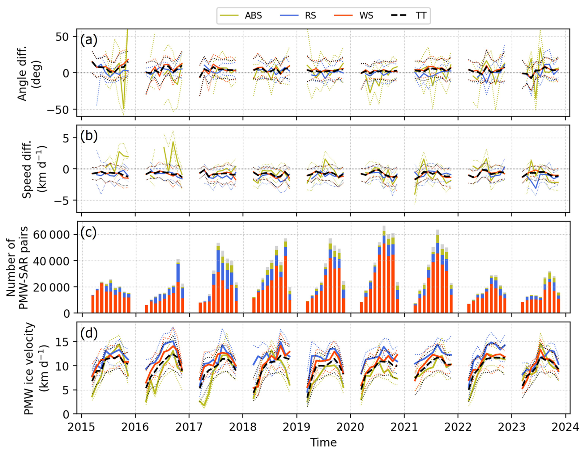
Figure 6 (a) Angle difference between PMW and SAR sea ice drift from 2015 to 2023 for Amundsen and Bellingshausen Sea (ABS), Ross Sea (RS), Weddell Sea (WS), and the entire Southern Ocean (TT). Positive angle difference indicates the PMW ice drift vector is clockwise rotated to the SAR ice drift vector, and negative angle difference means the anti-clockwise rotation of the PMW drift vector relative to the SAR ice drift vector. The solid lines indicate the monthly mean in each subregion, and the dashed lines indicate 25 % and 75 % quantiles. December, January, and February are excluded due to low sea ice coverage. (b) Speed difference between PMW and SAR sea ice drift from 2015 to 2023. (c) The number of PMW-SAR pairs used for the comparison. The colors of bars correspond to ABS, RS, and WS subregions, and the gray color represents the rest of the Southern Ocean. (d) Temporal variation of the mean sea ice velocity derived from PMW for each subregion. We note that only March–November results are presented due to the high uncertainty in sea ice drift during the austral summer months (December–February).

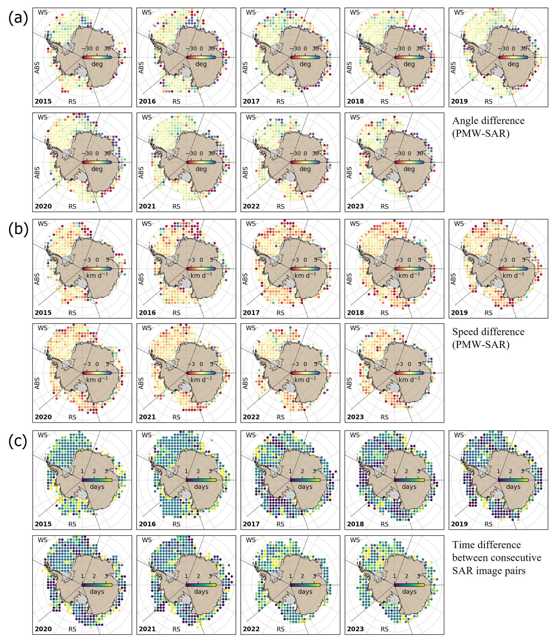
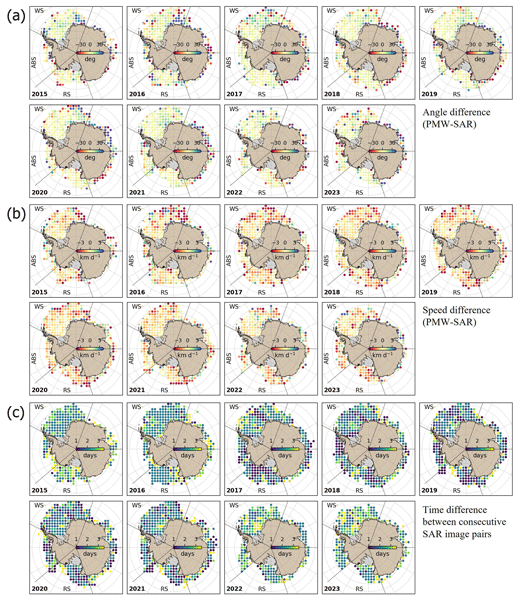
Figure 7 (a) Map of the angle difference between PMW and SAR sea ice drift from 2015 to 2023. Positive angle difference (bluish color) indicates the PMW ice drift vector is clockwise rotated to the SAR ice drift vector, and negative angle difference (reddish color) means the anti-clockwise rotation of the PMW drift vector relative to the SAR ice drift vector. (b) Map of speed difference between PMW and SAR sea ice drift from 2015 to 2023. (c) Map of the mean time difference between consecutive SAR image pairs for sea ice drift retrievals.

First, regarding the angle difference (Fig. 6a), the mean angle difference generally centers near zero, ranging from −20 to 20°. In both RS and WS, this angle difference remains consistent, without a significant temporal trend across months or years. The ABS sector shows somewhat larger fluctuations compared to the other regions, which might be attributed to the relatively lower number of comparison pairs available in this region (Figs. 6c and 7a). We also note that the angle difference appears relatively stable from 2017 to 2021, with fewer fluctuations in ABS. This stability potentially implies lower uncertainties in the SAR-derived sea ice velocity during these years, corresponding to the period when the full Sentinel-1A and 1B constellation was operational (April 2016–December 2021). As shown in Fig. 7c, the 2017–2021 period shows lower temporal gaps between SAR image pairs for drift retrievals, a factor that is known to reduce uncertainties in SAR-based sea ice drift. Regarding the spatial distribution of angle difference (Fig. 7), the majority of the WS, RS, and ABS sectors exhibit a mean angle difference within 20° (represented by yellowish colors). However, it is notable that the east WS consistently shows a slightly larger clockwise bias (bluish color) in the PMW sea ice drift relative to the SAR ice drift for all years.

The results of the speed difference show that the PMW sea ice drift tends to underestimate the SAR reference drift speed by 0.5–1.0 km d⁻¹ for all months from March to November throughout the entire 2015–2023 study period (Fig. 6b). Additionally, this 0.5–1.0 km d⁻¹ underestimation is consistent across all regions, including WS, RS, and ABS. While prior comparisons with buoy records only confirmed a similar underestimation tendency primarily around the WS sector due to limited buoy data availability, our extensive comparison with SAR sea ice drift demonstrates that this underestimation is a pan-Antarctic feature, prevalent across RS and ABS as well. This underestimation pattern is also observed in the annual maps of speed difference (Fig. 7b). Most of the Southern Ocean is characterized by a negative speed difference of 0–1 km d⁻¹ (reddish color), but this underestimation becomes more pronounced in the east WS and west RS, where the difference reaches approximately −3 km d⁻¹. Given that the east WS and west RS can be characterized as fast ice movement and dynamic ice edge conditions, we conjecture that the optimal interpolation is responsible for this large localized underestimation. We will provide a more detailed discussion on the impact of this interpolation method in Sect. 4.1.

4 Discussion

4.1 Impacts of interpolation

The uncertainty inherent in the NSIDC sea ice drift product is a composite of the errors stemming from (i) PMW feature tracking and (ii) the optimal interpolation used for gap filling and smoothing. In this section, we investigate the impact of the interpolation by comparing the raw PMW feature tracking velocity (PMW_raw), which is derived without optimal interpolation, against both buoys and the SAR-derived drift.

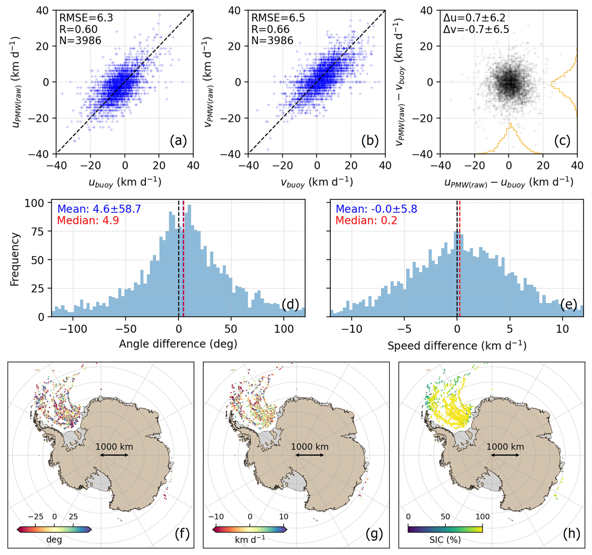
Figure 8 (a) Scatter plot between u-component sea ice drift from buoys and raw PMW feature tracking (without interpolation; PMW_raw), (b) scatter plot between v-component sea ice drift from buoys and PMW_raw. (c) Error distribution of the u and v sea ice drift components. (d) Distribution of angle difference and (e) speed difference between PMW_raw and buoy sea ice velocities. Location of buoys visualized by (f) angle difference, (g) speed difference, and (h) sea ice concentration.

Following the methodology of Sect. 3.2 (PMW-buoy comparison), we first compare the PMW_raw sea ice velocity with the buoy observations (Fig. 8). The PMW_raw product shows slightly lower RMSE for both u and v velocity components (around 6.3–6.5 km d⁻¹ RMSE), compared to the interpolated PMW product (Fig. 8a and b). More significantly, while the interpolated PMW product shows a negative speed bias (underestimation) of 2–3 km d⁻¹ relative to the buoys, the PMW_raw product shows virtually no speed bias, with a mean speed difference close to zero (Fig. 8e and g). For SIC > 85 %, PMW_raw exhibits only ∼ 0.6 km d⁻¹ of speed bias against buoy measurements. Furthermore, the PMW_raw drift demonstrates high directional accuracy, indicated by a mean angle difference of approximately 4–5° (Fig. 8d and f).

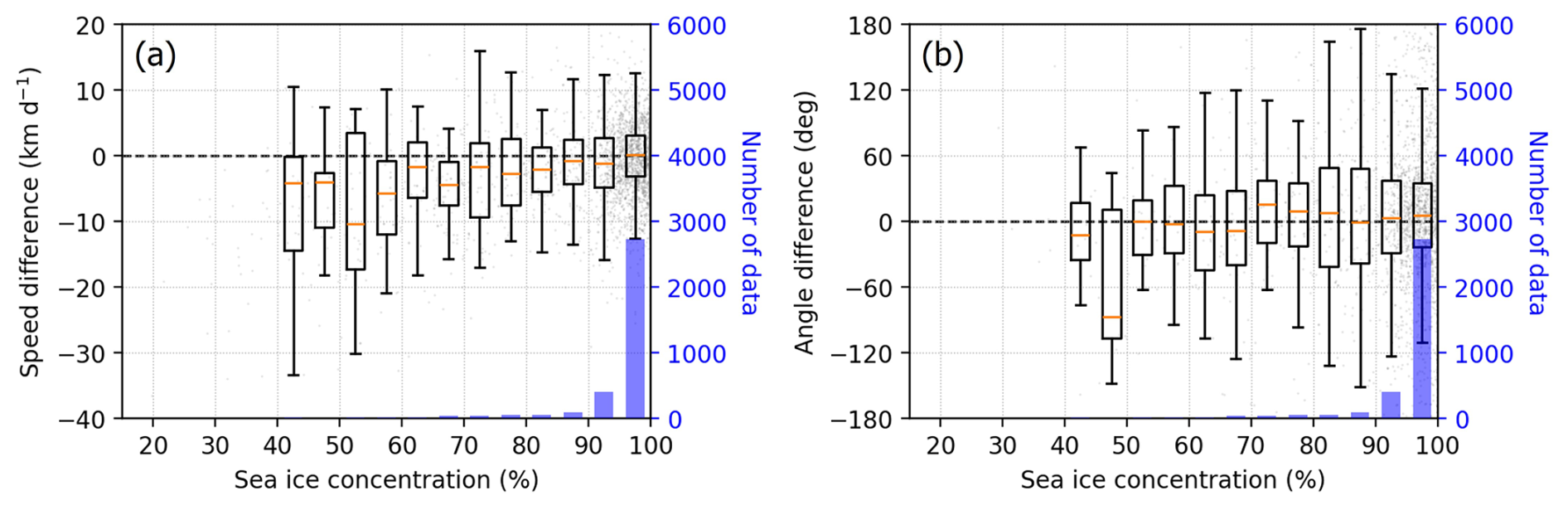
Figure 9 (a) Speed difference between raw PMW (without interpolation; PMW_raw) and buoy sea ice drift by sea ice concentration. (b) Angle difference between PMW_raw and buoy sea ice drift by sea ice concentration.

This compelling contrast demonstrates that the systematic underestimation of sea ice speed observed in the NSIDC Polar Pathfinder sea ice motion product is primarily attributed to the optimal interpolation scheme, rather than the intrinsic uncertainty of the PMW-based MCC feature tracking. However, we must note that the PMW_raw product still exhibits a tendency to underestimate sea ice speed under low SIC conditions (Figs. 9, 8g and h). Although PMW_raw comparisons are overwhelmingly concentrated in high-SIC areas (with SIC > 90 % in over 90 % of the total data points) (Fig. 9a), this residual bias implies that a feature-tracking-related bias remains. In low SIC areas, the PMW brightness temperature signal becomes increasingly contaminated by open-water emission, reducing the contrast and spatial coherence and making cross-correlation tracking challenging for coarse-resolution PMW images (Kwok, 2010). Similar to the interpolated PMW results, the PMW_raw sea ice drift direction remains robust and is not substantially affected by SIC conditions (Fig. 9b).

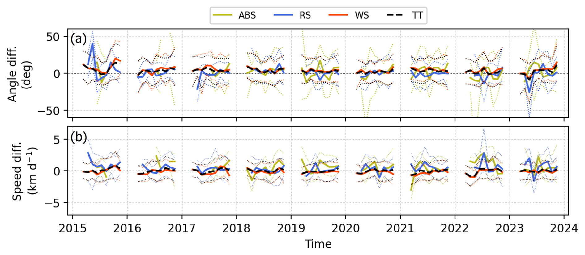
Figure 10 (a) Angle difference between PMW_raw and SAR sea ice drift from 2015 to 2023 for Amundsen and Bellingshausen Sea (ABS), Ross Sea (RS), Weddell Sea (WS), and the entire Southern Ocean (TT). The solid lines indicate the monthly mean in each subregion, and the dashed lines indicate 25 % and 75 % quantiles. (b) Speed difference between PMW_raw and SAR sea ice drift from 2015 to 2023. (c) The number of PMW_raw-SAR pairs used for the comparison. The colors of bars correspond to ABS, RS, and WS subregions, and the gray color represents the rest of the Southern Ocean.

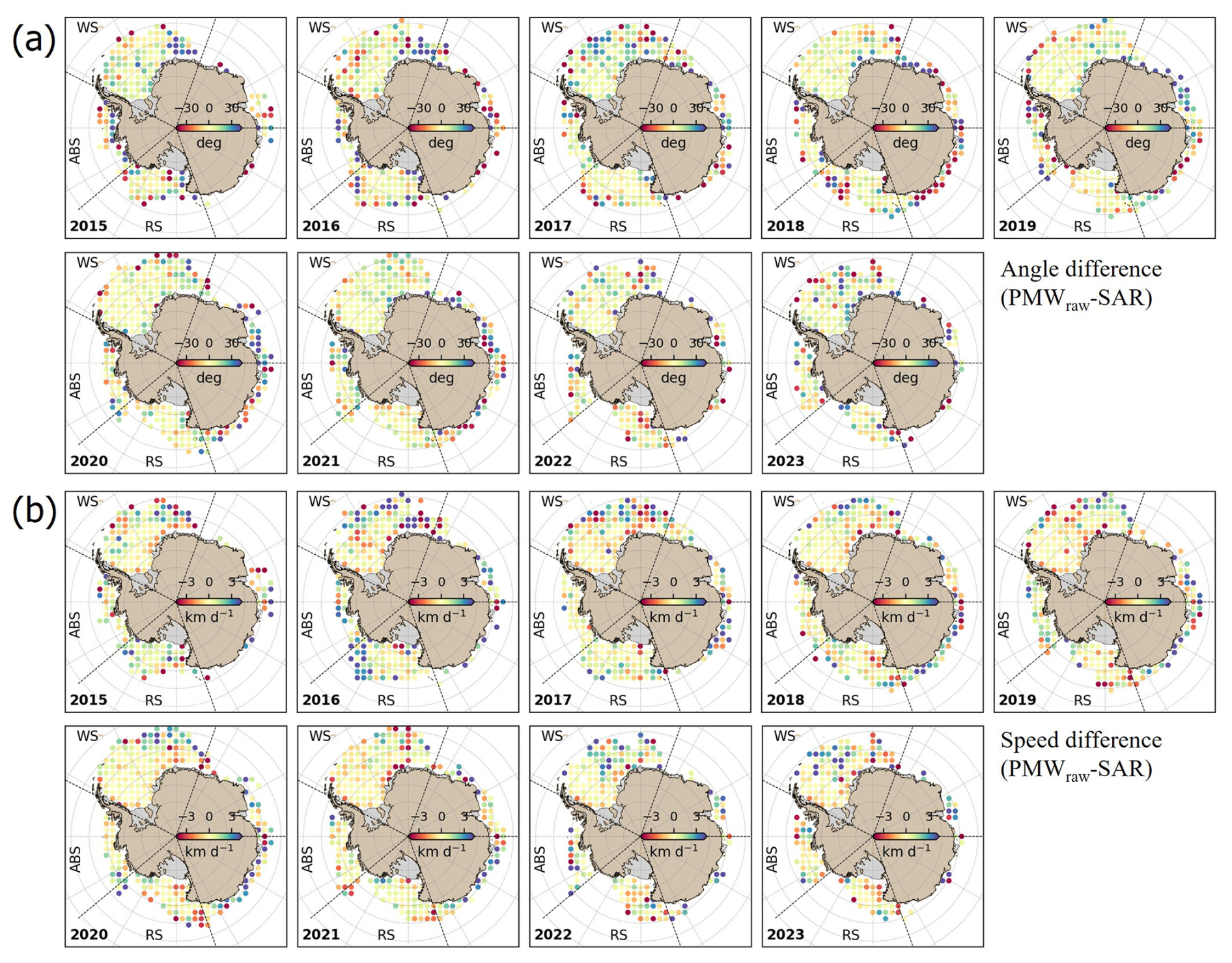
Figure 11 (a) Map of the angle difference between PMW_raw and SAR sea ice drift from 2015 to 2023. Positive angle difference (bluish color) indicates the PMW_raw ice drift vector is clockwise rotated to the SAR ice drift vector, and negative angle difference (reddish color) means the anti-clockwise rotation of the PMW_raw drift vector relative to the SAR ice drift vector. (b) Map of speed difference between PMW_raw and SAR sea ice drift from 2015 to 2023.

Similar results are observed in the comparison between PMW_raw and SAR sea ice drift (Figs. 10 and 11), further supporting the findings from the PMW_raw-buoy comparison. In terms of angle difference, the PMW_raw sea ice drift direction aligns well with the SAR sea ice drift, showing a near-zero mean angle difference within a range from −20 to 20°. Additionally, although a slight clockwise bias in the PMW_raw sea ice drift direction is still observed near the east WS, the magnitude of this bias is noticeably less severe than that found in the interpolated PMW product (Figs. 7a and 11a). On the other hand, in contrast to the systematic underestimation of the interpolated PMW sea ice drift speed (Fig. 6b), the mean speed difference for PMW_raw is close to zero, indicating no significant bias by time or region (Figs. 10b and 11b).

Table 1 Summary of sea ice velocity comparisons (angle and speed) for different dataset pairs.

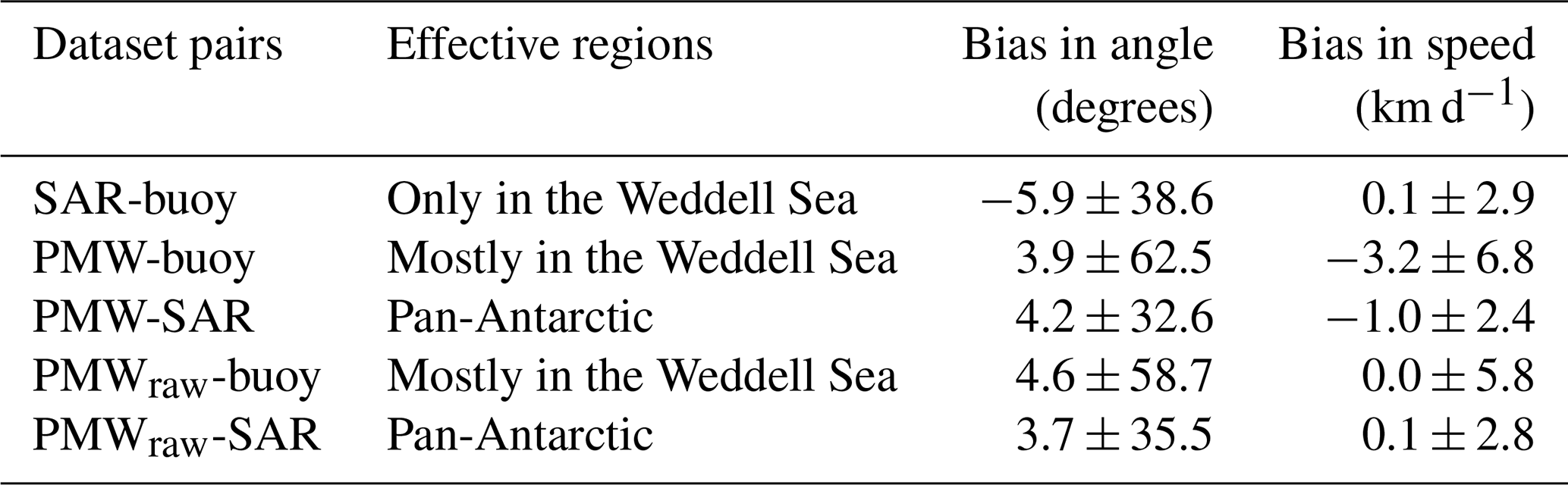
These extensive comparisons between PMW_raw and SAR sea ice drift strongly suggest that the PMW-based MCC feature tracking successfully reproduces sea ice velocity without a significant intrinsic speed bias, whereas the optimal interpolation systematically introduces a negative bias (i.e., underestimation of sea ice speed) into the final gridded sea ice motion product (Table 1). We propose two possible, non-exclusive reasons for the widespread underestimation of sea ice speed caused by the interpolation: (1) Smoothing effect: Optimal interpolation is designed to produce a smooth velocity field, which inherently acts to reduce the magnitude of real ice velocity, particularly in highly dynamic, higher-speed regions. (2) Bias at ice edge: Sea ice edges typically exhibit higher speeds than the middle of the ice pack. However, velocity at the ice edge is often estimated through interpolation of lower velocity values from the interior pack ice, leading to a substantial underestimation of the true speed near the ice edge.

4.2 Marginal ice zone and coastal region

Another critical aspect concerning the uncertainty assessment of the PMW sea ice drift product involves its proximity to the coast and the marginal ice zone (MIZ). Figure 12 illustrates the change in the PMW-SAR ice speed difference as a function of the distance to the ice edge and the coast for the WS, RS, and ABS sectors. In all three regions, the magnitude of the error in ice speed consistently increases when moving closer to the MIZ (particularly less than 200 km distance from the ice edge). Conversely, the error in ice speed appears to increase with increasing distance from the coast. However, given that greater distance from the coast often correlates with closer proximity to the MIZ, the relationship between ice speed difference and coastal distance is likely an indirect effect driven by the MIZ proximity. Therefore, this spatial analysis supports two key conclusions: (1) The uncertainty of the PMW-based interpolated sea ice velocity estimation significantly increases near the MIZ. (2) The proximity to the coast, after accounting for the MIZ relationship, does not significantly affect the uncertainty of PMW sea ice velocity.

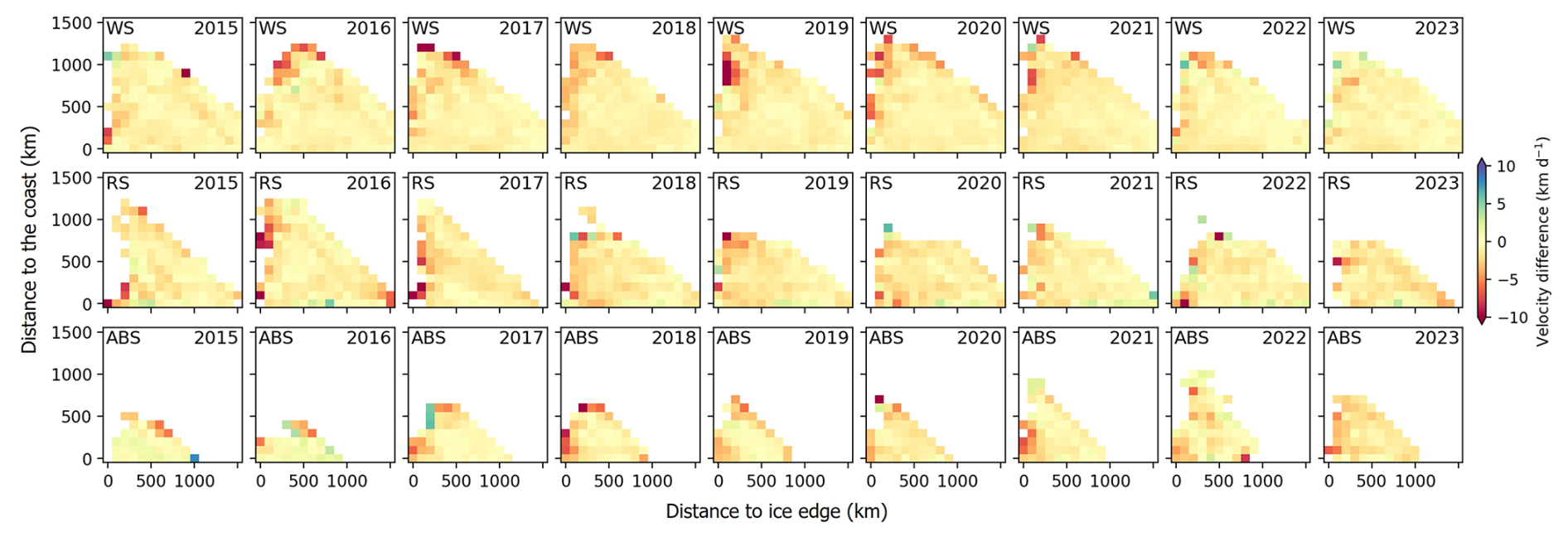
Figure 12 Speed difference between PMW and SAR sea ice drift by the distance to ice edge (x-axis) and coast (y-axis) for Weddell Sea (WS), Ross Sea (RS), and Amundsen-Bellingshausen Seas (ABS) from 2015 to 2023.

5 Conclusions

This study evaluates the uncertainty of the widely used Antarctic sea ice drift product derived from PMW observations (NSIDC Polar Pathfinder daily ice motion vectors, version 4) using both high-accuracy buoy data and high-resolution Sentinel-1 SAR imagery. The initial comparison with buoy data reveals significant errors in the PMW product, though spatially limited to the Weddell Sea. PMW-derived sea ice velocity has an uncertainty of 3.9±62.5° in drift direction and a substantial underestimation in drift speed, quantified as a mean difference of $-\mathrm{3.2}\pm \mathrm{6.8}$ km d⁻¹. In particular, this underestimation tendency is strongly dependent on sea ice concentration, resulting in a speed underestimation of approximately 10 km d⁻¹ in regions with < 50 % ice concentration. However, the drift direction shows no significant bias by ice concentration.

To overcome the spatial limitations of the buoy data, we establish the reliability of SAR-derived sea ice drift as a high-resolution reference. Compared with the buoy measurements, the SAR product achieved high accuracy, yielding RMSEs of 2.0 and 3.3 km d⁻¹ for the u and v velocity components, respectively. Vector metrics also confirm high accuracy of the SAR ice drift product, with an angle difference of $-\mathrm{5.9}\pm \mathrm{38.6}$°and a speed difference of 0.1±2.9°. This establishes the SAR product as a suitable high-resolution reference dataset for the pan-Antarctic assessment of the low-resolution PMW-derived sea ice drift.

Comparisons between PMW and SAR ice drift show that the ∼ 1 km d⁻¹ underestimation of drift speed is widespread across the Southern Ocean, including the Weddell Sea, Ross Sea, and Amundsen-Bellingshausen Seas, and persisted across the full study period (2015–2023). This negative speed bias was most pronounced in the east Weddell Sea and west Ross Sea, dynamic regions characterized by fast ice movement near the ice edges. In contrast, the PMW product successfully reproduced the overall drift direction with negligible bias, with the exception of a consistent 10–20° clockwise bias observed near the east Weddell Sea.

We identify the primary source of this widespread speed underestimation to be the optimal interpolation scheme used in the product generation. The raw ice speed derived solely from PMW-based feature tracking (PMW_raw) showed no significant speed bias relative to buoy and SAR data. We thus conclude that the optimal interpolation inherently smooths high-speed velocity gradients and fails to accurately capture the relatively high ice speed at the dynamic ice edge, leading to a systematic negative bias in the final product. Additionally, it should be noted that PMW_raw still exhibits a negative bias in ice speed in low-SIC areas due to contaminated open-water signals and relatively rapid thermodynamic and dynamic changes, such as ice formation, melt, and deformation.

This study underscores the importance of understanding the sources of uncertainty in widely used Antarctic sea ice velocity products, particularly those arising from data-processing stages. While the data production pipelines for the Arctic sea ice drift exhibit reliable quality due to relatively abundant input data, the Antarctic sea ice drift product remains subject to higher uncertainty due to data scarcity. Since the NSIDC sea ice velocity product provides uncertainty estimates associated with the optimal interpolation, users of this product must account for these uncertainties, particularly the underestimation in interpolated areas, in their scientific analyses. Based on this uncertainty assessment, we further recommend that future efforts to improve the Antarctic sea ice drift product should focus on advanced data fusion techniques that incorporate high-resolution velocity information from SAR and buoy measurements across the Southern Ocean to mitigate the smoothing and biases near the ice edge introduced by optimal interpolation.