Evaluation of ASCAT soil moisture retrievals and their potential to detect intraday variability

Accurate sub-daily soil moisture (SM) retrievals from satellite observations remain a major challenge due to sparse temporal sampling and retrieval uncertainties. This study introduces a localized convolutional neural network (CNN-l) framework designed to enhance SM estimates from Advanced SCATterometer (ASCAT) observations by exploiting spatial features and adapting to local conditions. The proposed approach achieves strong agreement with ERA5 reference SM, with total correlation coefficients exceeding 0.9, even at a sub-daily scale. Validation against in situ measurements from 568 monitoring sites across the contiguous United States (CONUS) shows a median temporal correlation of 0.65, compared to 0.59 for the operational ASCAT H120 product. Our CNN-based retrievals also reveal meaningful intraday variability when SM signals exceed retrieval uncertainty, particularly during heavy precipitation events (>10 mm d⁻¹), offering new insight into short-term hydrological responses. Future efforts should prioritize the integration of complementary satellite observations from multiple instruments to enhance retrieval accuracy, robustness, and temporal resolution. Additionally, strategies to improve retrieval of extremes (such as localization strategies or variable augmentation) should be further developed.

1 Introduction

Surface soil moisture (i.e., water in the top few centimeters of soil, hereafter referred to as SM) represents a relatively small component of the hydrological cycle (Trenberth et al., 2007), but plays a crucial role in land-atmosphere interactions and is vital for a variety of applications, including flood forecasting, agriculture, and water management (Bateni and Entekhabi, 2012; Ochsner et al., 2013; McColl et al., 2017). Reflecting its importance, significant efforts have been made to provide consistent SM datasets such as in situ SM measurements (e.g., through the International Soil Moisture Network, ISMN Dorigo et al., 2013, 2021), or SM estimates from satellite remote sensing (Aires et al., 2001; Kolassa et al., 2013; Araya et al., 2021; Singh and Gaurav, 2023; Han et al., 2023). Long-term operational products have been delivered by missions such as the European Remote Sensing satellite (ERS) scatterometer (Wagner et al., 1999a); Advanced SCATterometer (ASCAT) onboard the Metop satellites (Bartalis et al., 2007); the Soil Moisture and Ocean Salinity (SMOS) mission (Kerr et al., 2010); and the Soil Moisture Active Passive (SMAP) mission (Entekhabi et al., 2010). Apart from these SM products, directly retrieved from single satellite platforms, the European Space Agency Climate Change Initiative for Soil Moisture (ESA CCI SM) integrates these observations to obtain a consistent satellite-based long-term Climate Data Record (CDR) of SM (Dorigo et al., 2017).

While, historically, the retrieval of SM from active instruments (e.g., ERS and ASCAT) was partly based on a statistical approach (Wagner et al., 1999a), recent decades has seen a growing interest in employing purely statistical machine learning approaches for SM retrieval. Among these, neural networks (NNs) have emerged as powerful tools due to their ability to capture complex, nonlinear relationships between satellite observations and surface SM. Numerous studies have demonstrated the effectiveness of NNs in improving retrieval accuracy by exploiting large datasets and learning hierarchical representations of input features (Aires et al., 2001; Kolassa et al., 2017; Rodríguez-Fernández et al., 2017; Yao et al., 2021; Pellet et al., 2025), particularly for ASCAT observations (Aires et al., 2021a). Many existing retrieval products, however, operate at the pixel level (e.g., ASCAT soil moisture product and NN retrievals Aires et al., 2021a), neglecting the spatial dependencies present in satellite observations. Convolutional neural networks (CNNs) offer a promising alternative by exploiting spatial patterns, potentially improving retrieval performance beyond pixel-based approaches.

Despite extensive research on SM retrieval, most existing models operate at a daily temporal resolution, mainly due to high retrieval uncertainties (i.e., a low signal-to-noise ratio). Although daily estimates are sufficient for many applications, the availability of sub-daily (e.g., hourly) SM retrievals could unlock additional insights into dynamic processes such as soil-plant-atmosphere interactions, diurnal variation in evapotranspiration, and short-term hydrological forecasting (Vilà-Guerau de Arellano et al., 2020; Vermunt et al., 2022). However, relatively few studies have focused on this finer temporal scale (Kim et al., 2021; Wang et al., 2024). Notably, the Metop ASCAT CDR (EUMETSAT H SAF, 2021), which we use later in this study for comparison, already provides SM estimates at sub-daily resolution. Specifically, due to the orbital geometry of the ascending and descending passes, combined with the use of multiple ASCAT instruments (e.g., Metop-A and -B), a given location can be observed multiple times at different local overpass times on the same day. Here, we investigate whether a CNN-based approach can further enhance retrieval performance and better capture intraday variability.

This study aims to explore the potential of deep learning to improve sub-daily SM from ASCAT observations over the contiguous United States (CONUS). Although ASCAT provides global coverage, CONUS serves as an ideal study region because it features pronounced spatial and climatic variability (Bernhardt et al., 2018) and hosts a dense network of in situ measurements essential for robust validation. Specifically, we developed a localized convolutional neural network (CNN-l) framework designed to exploit spatial patterns and adapt to regional conditions, thereby reducing systematic biases.

The remainder of this study is organized as follows. Section 2 introduces the datasets employed in this study. Section 3 details the model architecture and evaluation metrics for sub-daily retrievals. Section 4 presents the model assessment, and Sect. 5 discusses its ability to capture intraday SM dynamics. Finally, Sect. 6 summarizes the findings and discusses implications for future applications.

2 Datasets

The core database used in this study consists of spatiotemporal coincidences of ASCAT level-2 observations and ERA5 reanalysis data (i.e., the fifth-generation ECMWF (European Centre for Medium-Range Weather Forecast) reanalysis Hersbach et al., 2023). Both datasets are projected onto a common 0.25° resolution grid covering the study domain, the CONUS, which spans from 125 to 70° W in longitude and from 25 to 50° N in latitude, encompassing a climatically diverse region (Bernhardt et al., 2018). The study period includes four years, from 1 January 2016 to 31 December 2019.

2.1 ASCAT information

ASCAT is a C-band (5.255 GHz) vertically polarized scatterometer known for its high radiometric accuracy (Figa-Saldaña et al., 2002). The ASCAT instruments are onboard three Metop-series polar-orbiting satellites, Metop-A, Metop-B, and Metop-C, launched on 19 October 2006, 17 September 2012, and 7 November 2018, respectively. These satellites operate in a sun-synchronous, low Earth polar orbit at an altitude of approximately 817 km, enabling near-global coverage every 12 h. In our study area, ASCAT measurements are typically acquired during two daily time windows: from 00:00 to 05:00 UTC (ascending orbits) and from 14:00 to 19:00 UTC (descending orbits). The ASCAT backscattering coefficient has been used to retrieve SM, as it is strongly influenced by the soil's dielectric properties, which vary with moisture content (Srivastava et al., 2009; El Hajj et al., 2016; Wagner et al., 2013, 1999b).

We used the Metop ASCAT SSM CDR (H120 version 7), which provides a consistent data record of SM-related products at 12.5 km resolution (EUMETSAT H SAF, 2021), covering the entire duration of Metop satellite missions (2007–present). This dataset is derived using the latest version of the SM retrieval algorithm developed by TU Wien under the EUMETSAT H SAF program (EUMETSAT H SAF, 2018). Two key variables are used here:

• Backscatter (σ₄₀). The ASCAT instrument measures backscatter at various incidence angles. To facilitate intercomparison and reduce vegetation-related effects, the Metop ASCAT CDR provides backscatter normalized to a reference incidence angle of 40° (in dB). This normalized value, σ₄₀, is more consistent and less sensitive to surface heterogeneity compared to raw backscatter observations.

• ASCAT surface soil moisture (SSM). The SSM or SM product represents the relative water content of the top few centimeters of the soil (approximately the top 5 cm). The retrieval algorithm scales the normalized backscatter (σ₄₀) between predefined dry and wet reference values to estimate the relative SM (EUMETSAT H SAF, 2018). These relative SM values are expressed as degrees of saturation, ranging from 0 % (completely dry) to 100 % (fully saturated).

The Metop ASCAT SSM CDR provides SM and σ₄₀ at the native temporal resolution of the satellite overpasses, without any temporal aggregation. The native spatial resolution of the ASCAT Level-1b product varies from 25 km (near swath) to 34 km (far swath). However, the CDR’s Level-1c and Level-2 products are resampled onto a discrete global grid with a uniform spatial sampling of 12.5 km in both latitude and longitude. To collocate ASCAT with ERA5 data, the CDR was regridded onto the ERA5 regular latitude-longitude grid at a 0.25° spatial resolution and resampled to an hourly temporal frequency.

To convert the relative SM values to volumetric SM (m³ m⁻³), we multiplied the ASCAT SM values by soil porosity, following the approach of Saxton and Rawls (2006). Porosity estimates were obtained from the Global Land Data Assimilation System (GLDAS) dataset (Rodell et al., 2004), accessible at https://ldas.gsfc.nasa.gov/gldas/soils (last access: 31 May 2025).

2.2 ERA5 database

In this study, we utilized the ERA5 reanalysis dataset to benefit from the comprehensive representation of the land-atmosphere system. Based on the ECMWF operational numerical weather prediction system, ERA5 incorporates a coupled land-atmosphere assimilation scheme that provides reliable datasets for our SM study. Since the original ERA5 data are available at an hourly resolution, they are used directly for our sub-daily SM retrieval.

Soil moisture (SM). ERA5 provides volumetric SM (m³ m⁻³) at 0–7, 7–28, 28–100, and 100–289 cm depths. To ensure consistency with ASCAT satellite measurements, we focus on the topmost layer of 0–7 cm, commonly referred to as surface SM. We use this variable as our primary target; owing to its spatial coherence and overall accuracy, it serves as a widely adopted benchmark in the development of machine-learning-based SM retrievals (Aires et al., 2005; Rodríguez-Fernández et al., 2019; Aires et al., 2021b; Pellet et al., 2025; Dinh, 2026).

Soil temperature (ST). ERA5 also offers ST at the same four depth intervals. As with ERA5 SM, we used the 0–7 cm layer to align with the surface sensitivity of the satellite observations. ST is considered an important auxiliary variable in SM retrieval, given its indirect relationship with soil water content through thermal properties (Campbell, 1985; Zhang et al., 2004).

Leaf area index (LAI). Vegetation structure significantly influences ASCAT backscatter-incidence angle (Petchiappan et al., 2022). Additionally, many previous studies have shown the usefulness of vegetation indices in SM retrieval (Aires et al., 2021a; Han et al., 2023; Pellet et al., 2025). Among various vegetation indices – such as the normalized difference vegetation index (NDVI) and enhanced vegetation index (EVI) – we selected the LAI. To maintain consistency with the ECMWF assimilation framework, we use the LAI forcing from ERA5 rather than externally sourced satellite datasets (Myneni et al., 2015; Yan et al., 2024). While ERA5 does not simulate dynamic LAI or assimilate LAI observations – relying instead on a prescribed monthly climatology (Duveiller et al., 2023) – using this specific background was necessary to ensure strict physical consistency with our training target.

The use of ERA5-derived ST and LAI as auxiliary inputs alongside ASCAT backscatter to predict SM introduces some dependence on the ERA5 framework. However, this design is both physically and methodologically justified. Physically, ST and LAI provide crucial boundary conditions that help the model separate SM effects from vegetation attenuation and thermodynamic variability in the ASCAT signal. Methodologically, they ensure the retrieval remains consistent with the ERA5 background space, a standard requirement for data assimilation (Rodríguez-Fernández et al., 2019). While the product inherits ERA5's large-scale statistics, its sub-daily and event-scale variations are driven by the independent ASCAT observations, capturing dynamic information absent from the ancillary variables alone.

2.3 In situ data from the International Soil Moisture Network

We used in situ SM data from the ISMN (Dorigo et al., 2013, 2021), which can be downloaded from https://ismn.earth/en/data/ (last access: 3 March 2025), to evaluate retrieval performance in 2019. The ISMN is a collaborative initiative supported by several international organizations and sustained through funding from the European Space Agency (ESA) and voluntary contributions from scientists and monitoring networks worldwide. It provides a consistent, globally accessible database of in situ SM measurements and serves as a key reference for validating both model-based and satellite-derived SM products (Kolassa et al., 2013; Batchu et al., 2023). This ISMN dataset was completely withheld from training, which enables a robust, independent evaluation of whether the retrieval effectively leverages ASCAT observations to generate physically meaningful SM estimates beyond the ERA5 background.

Within the study area, SM data from 568 in situ sites were extracted from three major networks: the Soil Climate Analysis Network (SCAN, Schaefer et al., 2007); the SNOwpack TELemetry (SNOTEL, Leavesley et al., 2010); and the United States Climate Reference Network (USCRN, Bell et al., 2013). Although many stations report SM profiles at multiple depths (up to 2 m), only the topmost measurement – taken at 0 to 7 cm depth – was used in this study for validation to align with the depth-sensitivity of ASCAT and ERA5 data. Sites with more than 100 d of missing observations in 2019 were excluded from the analysis. The in situ measurements are reported at hourly intervals and expressed in volumetric units (m³ m⁻³).

2.4 Other datasets

2.4.1 Land-cover data

To stratify retrieval performance across environmental conditions, we extracted the dominant land-cover type for each ISMN site using the 2019 National Land Cover Database (NLCD; USGS, 2024). This enables a targeted evaluation across major CONUS land-cover categories.

2.4.2 Precipitation data

To analyze model performance during rainfall events, we considered two precipitation datasets. First, ERA5 precipitation data is used to illustrate broad spatial patterns across CONUS. Additionally, we employed the Multi-Radar Multi-Sensor (MRMS) gauge-corrected quantitative precipitation estimation product (Zhang et al., 2016) to provide an independent, high-quality precipitation reference. By bias-correcting radar data with dense surface gauge networks, MRMS provides high-resolution (∼ 1 km, hourly) estimates that serve as a robust ground-truth proxy. For our analysis, these data were aggregated to a 0.25° grid to match our SM retrieval resolution.

3 Retrieval methods

3.1 Convolutional neural networks

CNNs, a class of deep learning models, were originally designed for tasks such as image and speech recognition (Lecun et al., 1998; Hinton et al., 2012). Due to their ability to efficiently process data with spatial or grid-like structures (i.e., images), CNNs have become increasingly popular in remote sensing applications for classification, segmentation, or retrieval (Maggiori et al., 2017; Rezaee et al., 2018; Aires et al., 2021a); see Ghanbari et al. (2021) for a meta-analysis.

CNNs operate on input data structured as multidimensional tensors. Here, input images are represented as a tensor X of dimensions (height) × (width) × (depth), where the height and width correspond here to 100×200 pixels, representing the spatial grid of latitude and longitude cells over the CONUS. The depth corresponds to the number of input channels, such as the backscattering coefficient σ₄₀ and other auxiliary variables. A CNN transforms these inputs through a series of layers, typically composed of convolution operations and nonlinear activation functions.

The core component of a CNN is the convolutional layer, which applies learnable kernels or filters – small matrices of weights, typically of size of $\mathrm{3}\times \mathrm{3}\times$ depth or $\mathrm{5}\times \mathrm{5}\times$ depth – across the input tensor. Each kernel performs an element-wise multiplication followed by a summation, effectively extracting localized spatial features. The result of this operation is a feature map. Multiple kernels are used per layer to learn diverse features.

Activation functions are applied after each convolution to introduce nonlinearity, which is crucial for learning complex patterns. The Rectified Linear Unit (ReLu), defined as $f\left(x\right)=max(\mathrm{0},x)$, is often used due to its computational efficiency and ability to mitigate vanishing gradient issues (Nair and Hinton, 2010; Goodfellow et al., 2016).

In addition, several architectural parameters influence the operations and outputs of convolutional layers:

• Stride determines the number of pixels the kernel moves at each step. Larger strides reduce the output resolution.

• Padding adds extra pixels around the border of the input image. “Same” padding preserves input dimensions, while “valid” padding does not, resulting in a smaller output.

While standard convolutions rely on weight sharing across the entire input, locally connected layers relax this constraint by applying distinct filters at every spatial location (Chen et al., 2015). This allows the network to learn location-specific patterns and achieve finer spatial specialization, driving their recent adoption in remote sensing applications (Boucher et al., 2023; Pellet et al., 2025).

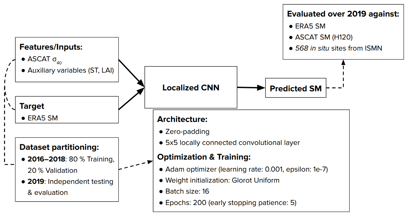
Figure 1 Workflow framework for ASCAT soil moisture (SM) retrieval, detailing the model inputs, localized CNN architecture, training parameters, and evaluation strategy.

3.2 Proposed model architecture

We consider a localized CNN variant, incorporating a locally connected convolutional layer in which filters learn distinct weights for each spatial location. To preserve spatial dimensions, zero-padding is applied prior to a single 5×5 locally connected layer without weight sharing. This localized architecture has been shown to perform particularly well in extreme cases (Dinh, 2026), motivating its use here for the sub-daily estimates. A detailed flowchart illustrating the proposed retrieval framework is provided in Fig. 1.

The input to the model comprises ASCAT-derived σ₄₀, along with two auxiliary variables – ST and LAI – identified in Sect. 2 as highly relevant to the target SM variable. While ST and LAI were selected for this study, other auxiliary variables, such as the antecedent precipitation evaporation index (Han et al., 2023) and the amplitude of the diurnal cycle of surface temperature (Prigent et al., 2005), may also contribute to SM retrieval. However, the selection and ranking of such variables fall outside the scope of this work.

Because the CONUS-scale dataset rendered computationally intensive automated optimization impractical (Rabiei et al., 2025), model hyperparameters were selected using a structured manual tuning approach. Consistent with methodologies established in recent remote sensing studies (Dinh, 2026), parameters were initially anchored to standard literature benchmarks (Rabiei et al., 2025; Pellet et al., 2025) and systematically refined against validation metrics until further adjustments yielded negligible improvements. Ultimately, our model is trained using the Adam optimizer (Kingma and Ba, 2017) with an initial learning rate of 0.001 and an epsilon value of 1 e⁻⁷ for numerical stability. Weight initialization is controlled using the Glorot Uniform initialization with a fixed random seed to ensure reproducibility. A batch size of 16 is used in the training. In addition, separate models are trained for ascending and descending satellite passes.

To robustly evaluate the model and actively prevent overfitting, we employed a strict temporal data splitting strategy alongside dynamic training constraints. The dataset spanning 2016 to 2018 is partitioned into 80 % for training and 20 % for validation, while the 2019 data is completely held out for independent testing and performance evaluation. During the training phase, overfitting is further mitigated through the implementation of early stopping; while the model is allowed to train for a maximum of 200 epochs, the process is halted early if the validation loss demonstrates no improvement over 5 consecutive epochs, at which point the optimal weights are restored.

3.3 Evaluation metrics

To evaluate the performance of SM retrievals, we used four statistical evaluation metrics: Pearson's correlation coefficient (r, unitless), root mean square error (RMSE, m³ m⁻³), and bias (Bias, m³ m⁻³). These metrics are computed as follows:

$$\begin{array}{}\text{(1)}& {\displaystyle }r={\displaystyle \frac{{\sum }_{i=\mathrm{1}}^N(y_{\mathrm{pred},i}-\stackrel{\mathrm{‾}}{y_{\mathrm{pred}}})(y_{\mathrm{ref},i}-\stackrel{\mathrm{‾}}{y_{\mathrm{ref}}})}{\sqrt{{\sum }_{i=\mathrm{1}}^N(y_{\mathrm{pred},i}-\stackrel{\mathrm{‾}}{y_{\mathrm{pred}}}{)}^{\mathrm{2}}}\sqrt{{\sum }_{i=\mathrm{1}}^N(y_{\mathrm{ref},i}-\stackrel{\mathrm{‾}}{y_{\mathrm{ref}}}{)}^{\mathrm{2}}}}}\text{(2)}& {\displaystyle }\mathrm{RMSE}=\sqrt{{\displaystyle \frac{{\sum }_{i=\mathrm{1}}^N(y_{\mathrm{pred},i}-y_{\mathrm{ref},i}{)}^{\mathrm{2}}}{N}}}\text{(3)}& {\displaystyle }\mathrm{Bias}={\displaystyle \frac{{\sum }_{i=\mathrm{1}}^N(y_{\mathrm{pred},i}-y_{\mathrm{ref},i})}{N}},\end{array}$$

where y_pred,i is the predicted SM, y_ref,i is the reference data (i.e., ERA5 or in situ SMs), N is the number of samples of SM data, and $\stackrel{\mathrm{‾}}{y_{\mathrm{pred}}}$ is the mean value of the predicted SM data. The standard deviation (SD, m³ m⁻³) of the difference between two datasets is also reported:

$$\begin{array}{}\text{(4)}& \mathrm{SD}=\sqrt{{\displaystyle \frac{{\sum }_{i=\mathrm{1}}^N(d_i-\stackrel{\mathrm{‾}}{d}{)}^{\mathrm{2}}}{N-\mathrm{1}}}}\end{array}$$

where $d_i=y_{\mathrm{pred},i}-y_{\mathrm{ref},i}$ is the difference between the predicted and reference SMs, and $\stackrel{\mathrm{‾}}{d}=\frac{\mathrm{1}}{N}{\sum }_{i=\mathrm{1}}^N{d}_i$.

4 Retrieval model assessment

As detailed in Sect. 3, we employed a localized CNN architecture that integrates three physically relevant inputs: σ₄₀, ST, and LAI. This configuration is denoted here as CNN-lo, where “l” indicates its localized setup and “o” refers to the orbit-based temporal alignment. The subsequent analysis assesses the performance of CNN-lo relative to ERA5 reanalysis and in situ measurements, and examines its improvements over the ASCAT H120 product.

All ASCAT overpasses (ascending and descending) were temporally collocated with the nearest hourly ERA5 reanalysis SM, hereafter referred to as ERA5-o. The corresponding ASCAT-based SM H120 product is denoted as H120-o. Likewise, in situ measurements (ISMN-o) were aligned to the closest ERA5-o timestamps to ensure consistent temporal reference across the datasets.

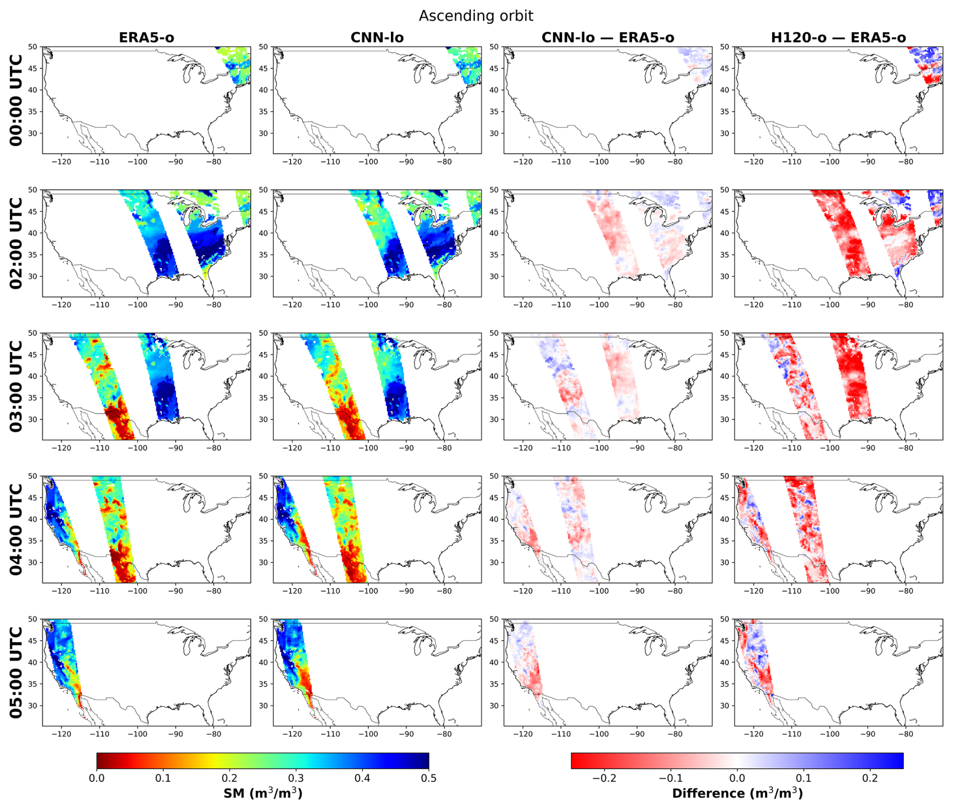
Figure 2 Hourly soil moisture (SM) estimates corresponding to five ascending ASCAT overpasses (00:00–05:00 UTC) on 20 January 2019. The first and second columns display SM values from ERA5-o and CNN-lo, respectively. The third column shows the SM differences between CNN-lo and ERA5-o, while the fourth column presents differences between H120-o and ERA5-o.

4.1 Evaluation against ERA5 SM

Figure 2 illustrates the ERA5-o and CNN-lo SM estimates and the difference between ASCAT-based retrievals (CNN-o and the H120 product) with respect to ERA5-o for multiple time slots on 20 January 2019, over ascending passes. Although separate models were trained for ascending and descending orbits, both are analyzed to maximize sub-daily coverage. In this example, five ascending and five descending (not shown) passes covered the study area, with each grid cell typically receiving up to two observations per orbit type – still limited, but sufficient to explore intraday variability under certain conditions.

The CNN-derived SM estimates show strong spatial consistency with the ERA-o reference, effectively capturing similar patterns and value ranges across all observed orbits (Fig. 2, first and second columns). This agreement is further reflected in the relatively small differences observed in the third column, where CNN-lo deviates minimally from ERA5-o. On the other hand, H120-o shows substantially larger discrepancies relative to ERA5-o, as indicated by the prevalence of dark red and blue regions in the fourth column. It should be noted that H120 was not trained on ERA5 and is therefore more independent of it than CNN-lo. Furthermore, the absolute spatial differences between H120-o and ERA5-o would be notably reduced if H120-o were rescaled to the ERA5 climatology using a cumulative distribution function (CDF) matching technique, rather than the current scaling based on saturated moisture content. When assessed over the full set of available orbits for the year 2019, CNN-lo achieves high correlation with ERA5-o (r=0.92 for ascending and r=0.91 for descending passes), confirming its ability to capture SM dynamics at sub-daily scales. In contrast, the H120 product achieves significantly lower correlations (r=0.58 and 0.59, respectively). Because ERA5 provides the most reliable estimates of SM (Aires et al., 2001), achieving comparable results using only ASCAT data in our retrieval is a promising outcome. For a more independent assessment, we next compare all products against in situ data.

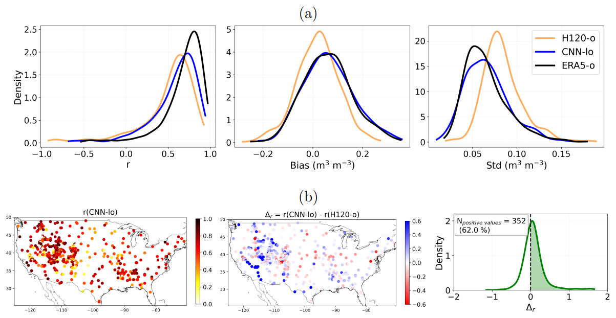
Figure 3 (a) Probability density functions (PDF) of temporal correlation (r), error bias (Bias, m³ m⁻³), and standard deviation of error (SD, m³ m⁻³) for ERA5-o, CNN-lo, and H120-o against in situ measurements at 568 sites across CONUS in 2019. (b) Maps showing (left) correlation of CNN-lo with in situ data and (middle) improvement in correlation with in situ data for CNN-lo relative to H120-o (Δ_r=r(CNN-lo) −r(H120-o)). Blue (red) indicates improved (degraded) correlation. The PDF of this Δ_r is also presented in the right panel.

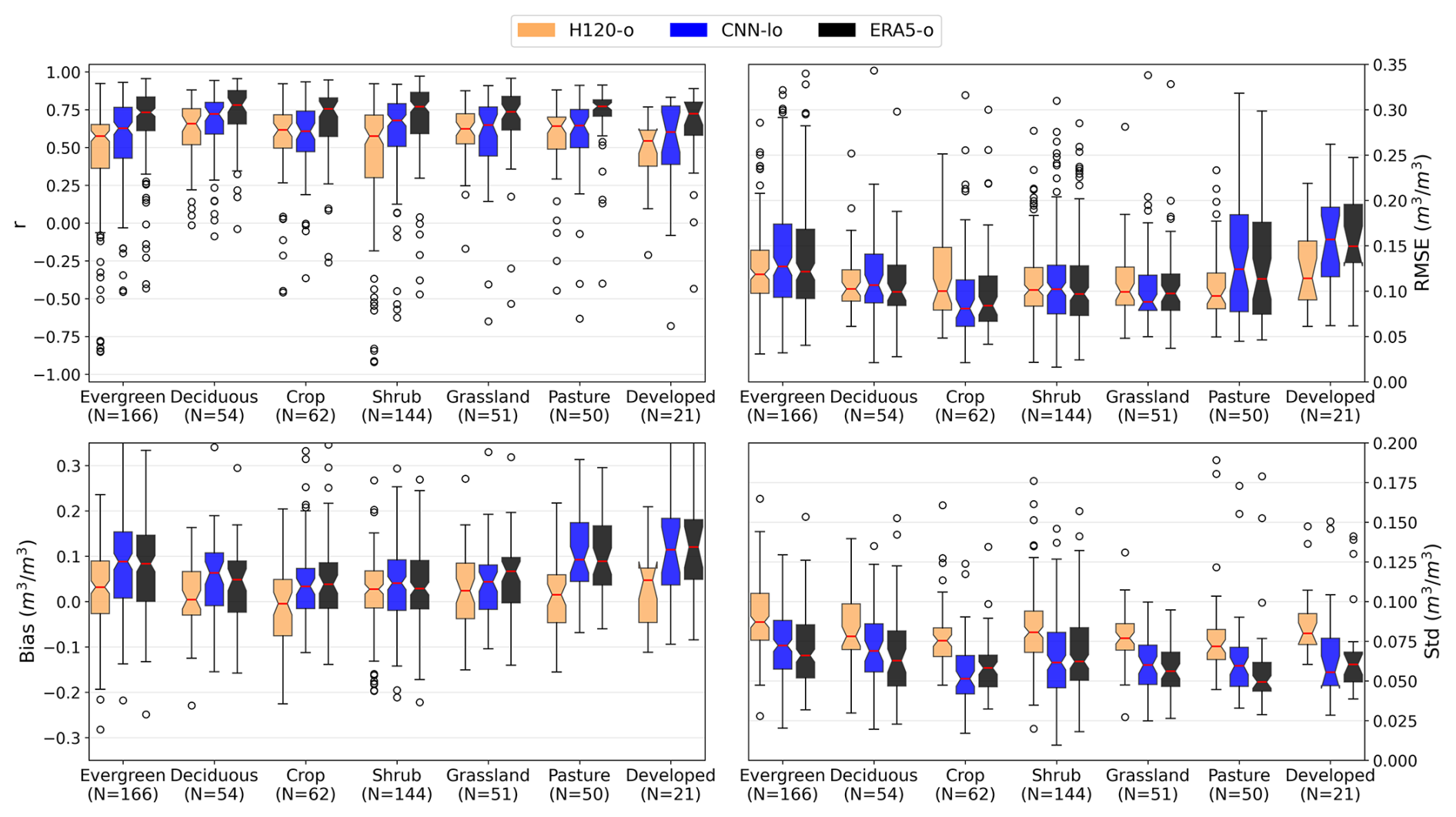
Figure 4 Boxplots of soil moisture (SM) retrieval performance (ASCAT H120-o, CNN-lo, and ERA5-o) compared to ISMN measurements. Results are grouped by major land-cover categories, including forests (evergreen, deciduous), crops, shrubs, grasslands, pasture, and developed areas. The number of sites within each class is shown in parentheses; underrepresented land-cover types (e.g., mixed forest, wetlands, barren, open water) are omitted.

4.2 Evaluation against in situ measurements

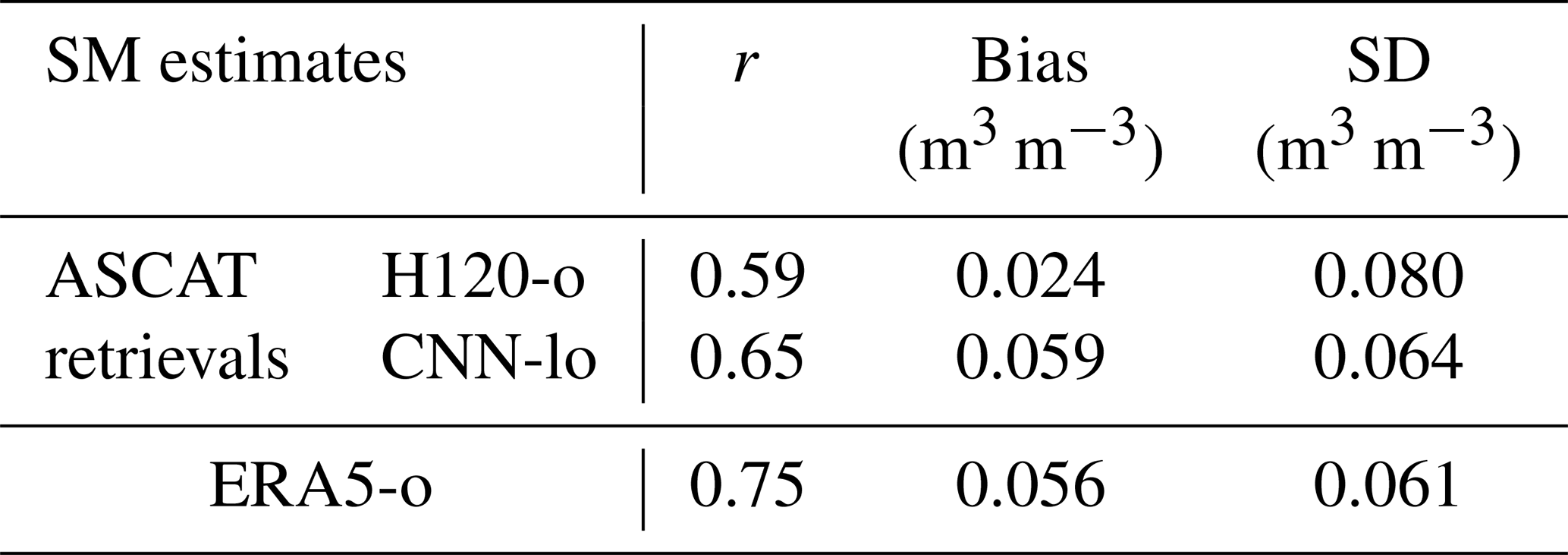
We evaluated three SM estimates (ERA5-o, CNN-lo, and H120-o) against measurements from 568 ISMN stations across CONUS in 2019 (see Sect. 2). Each ISMN station was collocated to the nearest 0.25° grid cell to match the resolution of the gridded SM estimates. Table 1 presents the performance metrics, and Fig. 3a presents probability density functions (PDFs) of temporal correlation (r), bias (Bias, m³ m⁻³), and standard deviation (SD, m³ m⁻³). ERA5-o achieves the highest overall agreement with in situ data (median r=0.75, Bias =0.056, and SD =0.061), which is expected given that ERA5 assimilates a wide range of satellite observations and in situ measurements. ERA reanalysis has long been shown to yield higher SM accuracy than any individual satellite retrieval (see, for instance, Aires et al., 2001). The H120 product shows the lowest median correlation (r=0.59) and exhibits a long negative tail in the bias distribution, despite having the lowest median bias error (0.024 m³ m⁻³). Its higher error variability (SD) indicates reduced skill in capturing SM dynamics. CNN-lo significantly outperforms H120, achieving a median correlation of 0.65 and error levels comparable to ERA5, as shown in the distributions in Fig. 3a.

Table 1 Performance metrics (median values across 568 sites) for soil moisture (SM) retrievals (ASCAT H120-o, CNN-lo, and ERA5-o) evaluated against ISMN in situ data for 2019. Metrics include temporal correlation (r), bias, and standard deviation (SD).

The spatial distribution of correlation coefficients (Fig. 3b) indicates that CNN-lo generally performs well, with particularly strong agreement in the western and southeastern regions. The difference map of Δ_r (middle panel) demonstrates that CNN-lo improves upon H120-o in a large part of the domain, as indicated by the predominance of blue points. Quantitatively, CNN-lo outperforms H120-o at 352 of 568 sites, about 62 % (green area in the last panel of Fig. 3b). The PDF of Δ_r further confirms this improvement, showing a pronounced positive tail approaching 2. This pattern reflects substantial performance gains at many sites where H120-o exhibits a low or even negative correlation. Although about 38 % of the sites show a reduced correlation, the magnitude of these degradations is generally much smaller than the observed improvements.

Evaluating performance across major CONUS land-cover classes (Fig. 4) confirms trends seen in Table 1 and Fig. 3: while H120-o achieves lower biases across all classes – an artifact of local calibration (Aires et al., 2021b) – it yields higher standard deviations. Regionally, H120-o shows marginally better correlations than CNN-lo for croplands, reflecting results over the central Great Plains in Fig. 3b. Conversely, CNN-lo excels over complex topography (e.g., the mountainous western US), outperforming H120-o in correlation over evergreen and deciduous forests due to its ability to leverage spatial context (Pellet et al., 2025). Despite being trained on ERA5, CNN-lo outperforms its training target over crops and grasslands in terms of correlation.

To better illustrate the comparison at the site level, Fig. 5 shows hourly SM time series for six randomly selected ISMN sites. All products capture the temporal dynamics and amplitude of SM reasonably well. ERA5-o consistently achieves the highest correlations (>0.8), reflecting the advantage of assimilating multiple data sources. CNN-lo closely tracks the ERA5 SM ranges and temporal patterns. The H120 product exhibits higher temporal variability than the other retrievals.

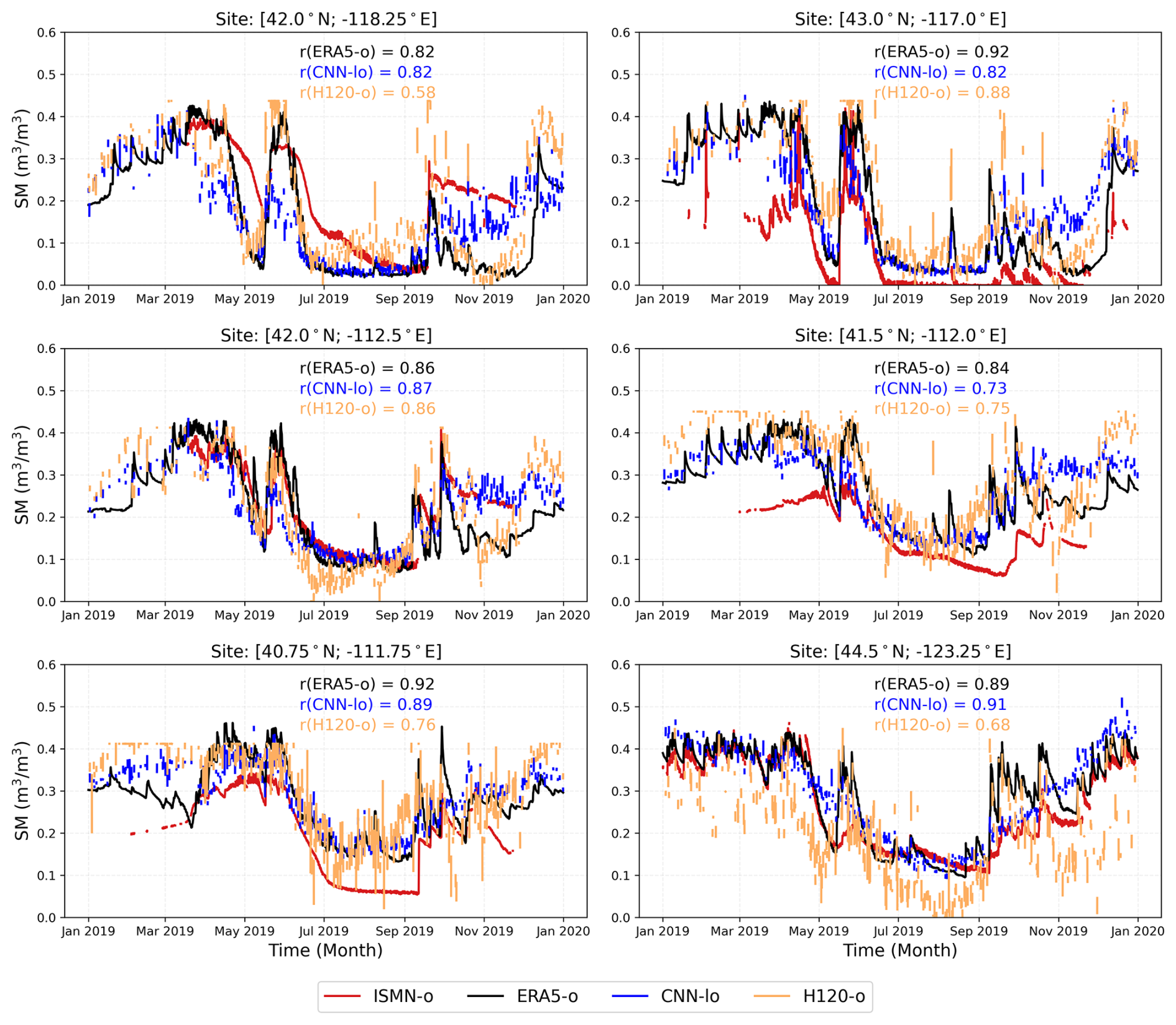
Figure 5 Hourly soil moisture (SM) time series in 2019 at six sites, comparing in situ data (ISMN-o) with ERA5-o, CNN-lo, and ASCAT H120 product (H120-o). Each panel includes the temporal correlation coefficient (r) between each SM estimate and in situ measurements.

5 Analysis of intraday variability

The previous section demonstrated that CNN-lo outperforms the ASCAT H120 product, exhibiting strong agreement with both ERA5 and in situ measurements. Here, we investigate the capability of this NN-based approach to capture diurnal SM variations, despite the inherent limitation in the satellite sampling frequency. Since only a few satellite observations are available per pixel per day (e.g., Fig. 2), extracting a reliable diurnal signal is challenging.

5.1 Analysis of one case study

To illustrate the capacity of CNN-lo to capture short-term SM dynamics, we analyzed a day with a significant precipitation event: 20 November 2019. Figure 6a displays spatial maps of daily SM amplitude (Δ_SM) derived from CNN-lo and ERA5-o. For reference, the full 24 h SM amplitude of ERA5 (ERA5-24h) and the corresponding daily accumulated precipitation are also represented. High Δ_SM values appear in the southwest region, coinciding with a precipitation event captured in the ERA5 precipitation data.

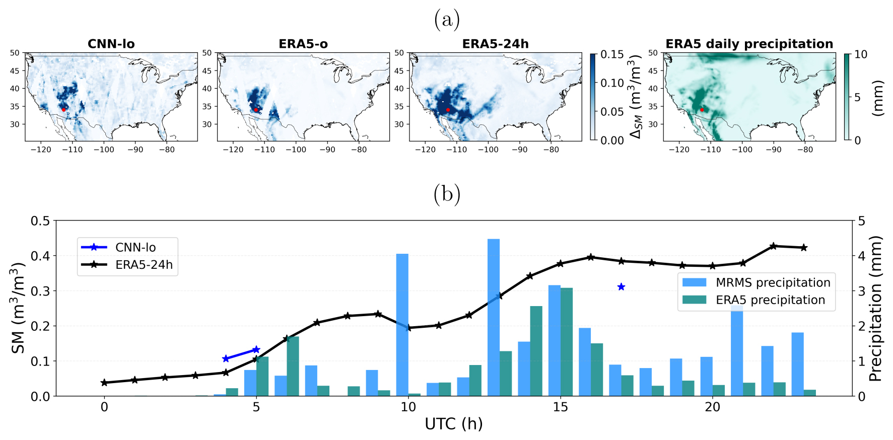
Figure 6 (a) Maps of daily SM amplitude (Δ_SM) on 20 November 2019, derived from CNN-lo and ERA5-o. ERA5-24h (full 24 h amplitude) and daily accumulated precipitation are also shown for reference. (b) Hourly SM time series at [34° N, 112.75° W] (marked with a red dot in the maps), comparing CNN-lo retrievals to ERA5-24h. CNN-lo estimates correspond to three ASCAT overpasses: two ascending (04:00–05:00 UTC) and one descending (17:00 UTC). Precipitation data from both the independent MRMS gauge-corrected product and ERA5 are also presented.

We then examined the hourly SM time series in a representative grid cell located at [34° N, 112.75° W], shown in red in Fig. 6a. To independently evaluate the SM dynamics, we incorporated the MRMS gauge-corrected precipitation product, spatially aggregated to match our target grid cell. As shown in Fig. 6b, according to both MRMS and ERA5 precipitation datasets, the rain started around 04:00 UTC and continued throughout the day. Prior to rainfall (00:00–04:00 UTC), ERA5 SM values remained low, then gradually increased, reaching approximately 0.42 m³ m⁻³ by the end of the day.

On this day, ASCAT provided three overpasses: two during the ascending orbit (04:00–05:00 UTC) and one during the descending orbit (17:00 UTC). CNN-lo retrieved SM estimates for these overpasses, showing good agreement with ERA5. The CNN-lo daily SM amplitude (Δ_SM=0.2 m³ m⁻³) is significant but lower than ERA5-24h (0.31 m³ m⁻³). The errors are due to (1) retrieval uncertainties and (2) limitations in temporal sampling.

While a single case study cannot serve as a formal demonstration of the model's overall capability, this example illustrates the model's ability to capture intraday SM dynamics during heavy precipitation events, despite sparse ASCAT observations. Crucially, the alignment with independent MRMS precipitation data confirms that the retrieved SM response is physically consistent with actual observed rainfall, rather than merely reflecting the ERA5 forcing. Capturing these dynamics is critical for hydrological applications, as rapid soil saturation can provoke flood risks. However, the spatial depiction of intraday variability remains strongly constrained by ASCAT's sampling frequency. Integrating observations from multiple instruments (e.g., SMOS, SMAP) is expected to enhance both retrieval accuracy and temporal resolution in future work.

5.2 Δ_SM sensitivity to precipitation level

The key question is: What level of intraday SM variation can be reliably detected from NN-based retrieval? To address this, we compared the diurnal SM amplitude (Δ_SM) from CNN-lo with ERA5-o for all pixels and days in 2019 having at least two ASCAT observations. Results are shown in Fig. 7.

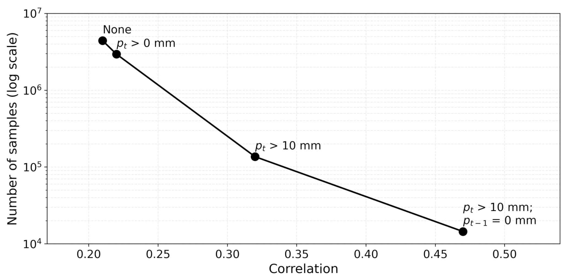
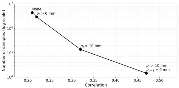
Figure 7 Correlation between diurnal SM amplitude (Δ_SM) estimated by CNN-lo and the ERA5-o reference as a function of daily precipitation thresholds (p_t in mm, where t denotes the day index). “None” indicates no threshold applied. The x-axis presents the correlation values, and the y-axis shows the corresponding number of samples on a logarithmic scale for each threshold condition.

When considering all 4 419 791 samples (i.e., threshold is none), the correlation between CNN-lo and ERA5-o Δ_SM is modest (r=0.21), indicating that most observed differences reflect retrieval noise rather than true diurnal variability. This is expected given ASCAT's sparse temporal sampling and the inherent difficulty of resolving small sub-daily changes. However, as shown in Sect. 5.1, to isolate such cases, we progressively applied precipitation thresholds. For days with any measurable rainfall (p_t>0 mm), correlation improves slightly to 0.22. For heavier events (p_t>10 mm), correlation rises to 0.32, and further increases to 0.47 when excluding cases with rain on the previous day ($p_{t-\mathrm{1}}=\mathrm{0}$ mm). This subset (14 445 samples) primarily reflects isolated heavy rainfall events, suggesting that CNN-lo can capture SM responses when the signal-to-noise ratio is favorable.

Figure 8 shows the scatter plots for this subset (p_t>10 mm, $p_{t-\mathrm{1}}=\mathrm{0}$ mm), comparing CNN-lo and ERA5-o for: (1) maximum SM value (SM_max), (2) minimum SM value (SM_min), and (3) diurnal SM amplitude (Δ_SM). Each point represents one single pixel-day. CNN-lo tends to underestimate SM_max and slightly overestimate SM_min – a typical behavior of statistical models that dampen extremes (Hastie et al., 2009). Despite this, strong agreement with ERA5-o is achieved for SM_max and SM_min (r=0.82 and r=0.88, respectively). As expected, Δ_SM exhibits lower correlation (r=0.47) because amplitude errors propagate from both extremes. The third panel of Fig. 8 indicates that the regression fit (dashed red line) is skewed by high-amplitude cases. However, the denser cluster of points in the 0–0.05 m³ m⁻³ range (i.e., yellow points) suggests that the model captures stable SM conditions well. These low-amplitude cases likely correspond to days with minimal diurnal variation, where the model performs more reliably.

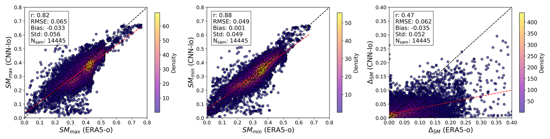
Figure 8 Scatter plots comparing CNN-lo and ERA5-o SM for days with isolated precipitation events (p_t>10 mm and $p_{t-\mathrm{1}}=\mathrm{0}$ mm) in 2019. Panels show: (1) maximum SM value (SM_max); (2) minimum SM value (SM_min); and (3) the resulting diurnal SM amplitude (${\mathrm{\Delta }}_{\mathrm{SM}}={\mathrm{SM}}_{\max }-{\mathrm{SM}}_{\min }$), all in m³ m⁻³. Each point represents one pixel-day. Statistical metrics include total correlation (r), root mean square error (RMSE, m³ m⁻³), bias (Bias, m³ m⁻³), standard deviation (SD, m³ m⁻³), and number of samples (N_samples). The dashed black line represents the 1:1 line; the red dashed line is the linear regression fit. The colorbar indicates the local density of dots in the scatterplot.

5.3 Evaluation of intraday SM variations

We now examine the spatial and temporal structure of these intraday variations over the CONUS. Figure 9 summarizes key intraday SM signals for the 14 445 cases identified above: timing of SM_max and SM_min, their respective values, and the diurnal amplitude Δ_SM for CNN-lo, ERA5-o, and ERA5-24h. Note that higher precipitation is concentrated in the eastern CONUS, resulting in limited sampling in western regions (white pixels).

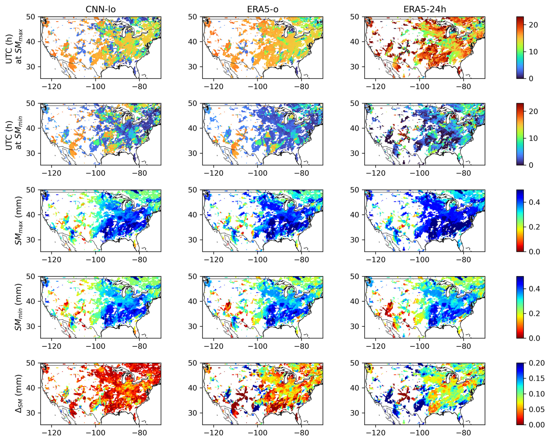
Figure 9 From top to bottom: (1) Time of maximum SM in UTC (h); (2) time of minimum SM in UTC (h); (3) maximum SM value (SM_max, m³ m⁻³); (4) minimum SM value (SM_min, m³ m⁻³); and (5) diurnal SM amplitude (Δ_SM, m³ m⁻³). Columns represent CNN-lo (left), ERA5-o (middle), and ERA5-24h (right). Only days in 2019 with total daily precipitation exceeding 10 mm and no rainfall on the preceding day are included (i.e., 14 445 selected cases). Each pixel reflects the average signal computed over all available days.

CNN-lo and ERA5-o exhibit similar spatiotemporal patterns. Note, however, that the estimation of the SM maximum and minimum times is degraded when limited by the ASCAT time sampling. For CNN-lo and ERA5-o, in the eastern part, SM typically reaches its maximum in the late afternoon (around 17:00 UTC) and its minimum in the early morning (around 03:00 UTC), aligning with ASCAT overpass times. In contrast, ERA5-24h – benefiting from full hourly coverage – shows SM_max occurring later in the evening and SM_min earlier, indicating a more complete description of the diurnal cycle.

Maps of SM_max and SM_min are largely consistent across CNN-lo and ERA-o, supported by the high correlation reported in Fig. 8. However, CNN-lo underestimates Δ_SM compared to ERA5-o, consistent with the tendency of statistical models to dampen variability (Hastie et al., 2009; Skafte et al., 2019). Interestingly, ERA5-o also exhibits lower amplitudes relative to ERA5-24h, which has a broader dynamic range due to full diurnal coverage. Therefore, the underestimation by CNN-lo likely reflects both retrieval smoothing and ASCAT's temporal sampling limitations – a constraint that could be mitigated through multi-sensor data fusion, as discussed in Sect. 6.

6 Conclusion and perspectives

This study demonstrates that a localized CNN can improve SM retrieval from ASCAT observations. The CNN approach achieves correlations exceeding 0.9 with ERA5 and a median temporal correlation of 0.65 against in situ measurements – outperforming the ASCAT H120 product (0.58 and 0.59, respectively). Importantly, we show that intraday SM signals are detectable under specific conditions, particularly when the diurnal amplitude (Δ_SM) exceeds retrieval uncertainty. Such favorable signal-to-noise conditions typically occur during intense precipitation events over unsaturated soils. These findings reveal a pathway toward sub-daily SM monitoring, with direct value for hydrological forecasting, agricultural management, and early-warning systems (Brocca et al., 2010; Vilà-Guerau de Arellano et al., 2020; Vermunt et al., 2022).

Despite this promise, significant challenges remain. Firstly, like most statistical models, CNN retrievals tend to attenuate extreme values, leading to an underestimation of Δ_SM (Hastie et al., 2009). Future work should explore architectures better suited for nonlinear dynamics, potentially through enhanced localization strategies or input feature augmentation (Boucher and Aires, 2023). For instance, including soil texture, precipitation-related data, or other auxiliary variables may further improve retrieval skill, given their strong relationship with SM (Abbaszadeh et al., 2019). Additionally, integrating dynamic components (O and Orth, 2020) into the retrieval framework could enable better representation of temporal dependencies, thereby improving overall model accuracy at sub-daily scales.

Secondly, the temporal sampling of satellite observations remains a major limitation. In our example of ASCAT observations, with typically two overpasses per day per orbit type, key intraday dynamics are easily missed. Multi-sensor integration offers a potential solution, but it introduces additional complexity, such as inter-sensor calibration, heterogeneous retrieval uncertainties, and the need for temporal regularization (Samadzadegan et al., 2025). Conditioning retrievals on external information, such as precipitation or other ancillary information, could also improve sensitivity to rapid SM changes. Advances in machine learning, such as foundation models, may facilitate these developments by enabling integration of heterogeneous data sources, dynamic downscaling, and spatiotemporal consistency (Hong et al., 2024; Yu et al., 2025).

Beyond SM, the proposed CNN framework has broader applicability for retrieving geophysical variables characterized by spatial structure and incomplete radiative transfer constraints, such as land surface temperature, surface emissivity, vegetation cover, and surface water extent. Moreover, these methods could extend to forward modeling, such as predicting satellite brightness temperatures directly from geophysical states. By leveraging spatial patterns and localized adaptation, deep learning provides a powerful approach to increasing the spatiotemporal fidelity of remote sensing products. Such downscaling enables real-time environmental monitoring at previously unattainable scales.