A neural-network based observation operator for the assimilation of microwave satellite observations with LDAS-Monde on global cropland for improving land-surface variables

The knowledge of land-surface variables (LSVs) is essential for an accurate description of the carbon cycle and, hence, for deriving the fraction of anthropogenic CO₂ emissions contributing to global warming. For a better representation of LSVs like the leaf-area index (LAI), we assimilate the observations of the satellite microwave sensors SMAP and AMSR2 with our land-data assimilation system (LDAS) on global cropland. Dedicated observation operators using a neural network (NN) are developed to enable a direct assimilation of the measured brightness temperatures. Direct assimilation is not yet an established method due to the incomplete representation of physical emission processes and the associated computational constraints of physical observation operators. We derive an optimal set of predictors for both instruments resulting in a good match between model equivalent and the observations in the testing period, with correlations up to 0.87/0.93 and a total RMSE of 8.2/3.6 K for SMAP/AMSR2, respectively. The implementation of the derived weights into the LDAS is straightforward and is found to lead to a reasonably good performance of the assimilation system, with a stronger improvement of the departures for SMAP than for AMSR2, which can be attributed to the characteristics of the microwave bands of the observations. For the best assimilation experiments, the verification against LAI observations shows an improvement compared to the open loop on a global scale. In agricultural regions of the world that are particularly susceptible to drought, AMSR2 experiments outperform SMAP experiments in terms of LAI in most cases. We also investigated the impact on the Gross Primary Productivity (GPP) and soil-water index (SWI) anomalies and found relatively little impact with mixed results. Nevertheless, the seasonal and sub-seasonal variability is still not well represented due to systematic errors in our land surface model.

1 Introduction

With climate change being one of the most important challenges of our time, accurate climate projections are essential. For those, the knowledge of the current state of the main drivers of the global warming is needed and, hence, not only the increase of atmospheric species contributing to the greenhouse effect but also the fraction of both biogenic and anthropogenic greenhouse gases therein. As a consequence, the EU-funded project CORSO (https://www.corso-project.eu/, last access: 3 November 2026), where this study is part of, aims at providing a continuous monitoring of land surface variables, which allows for an improved estimation of the carbon cycle and, eventually, the biogenic CO₂ emissions.

With data assimilation (DA), the initial state of the variables of interest can be optimised by ingesting relevant observations. Especially for LSVs, the availability of microwave-satellite instruments that observe in near-real time and provide data resampled on a grid covering the entire globe offers the opportunity to improve the state of the model variables (Walker and Houser, 2001; Reichle, 2005; Pauwels et al., 2007; among others).

Frequently, assimilation systems rely on retrieved data products (e.g., Dente et al., 2008; Jarlan et al., 2008; Draper et al., 2012) but with radiative transfer models (RTMs) becoming more accessible and efficient, the direct assimilation of brightness temperatures (T_b) using an RTM-based observation operator is often preferred (Reichle et al., 2021; Vural et al., 2023; Kolassa et al., 2025) as it avoids inconsistencies added by simplifications required by the retrieval method.

As the main difficulty of transforming model variables to observation space to obtain the so-called model equivalent remains, recent approaches include the exploitation of different algorithms of machine learning, especially neural networks (Xue and Forman, 2015; Corchia et al., 2023; De Gélis et al., 2025). These methods are usually resource-intensive in the training part but the actual application of the training results as observation operator is generally straightforward and computationally significantly less expensive than RTMs.

While the assimilation of NN-based retrievals has been established (e.g., Rodríguez-Fernández et al., 2019, on SMOS; Kolassa et al., 2017, on SMAP; and Rodríguez-Fernández et al., 2016, on AMSR-E), SMAP brightness temperatures were also assimilated directly by Reichle et al. (2023) and Kolassa et al. (2025) using a tau-omega RTM with local calibration (De Lannoy et al., 2013), which led to a general benefit on the numerical weather prediction (NWP), including the representation of a tropical cyclone.

Although mostly used for retrieving soil moistures (SMAP; Soil Moisture Active Passive) or atmospheric variables (AMSR2; Advanced Microwave Scanning Radiometer), microwave observations can also be assimilated to improve variables related more closely to vegetation since it is responsible for absorption of the radiation before it reaches the ground. Kumar et al. (2020) improved the estimate of evapotranspiration and the GPP by the assimilation of vegetation optical depth (VOD) derived from SMAP and AMSR2 over the United States. Similarly, Mucia et al. (2022) assimilated surface soil moisture, LAI, and VOD derived from different microwave bands and found improvements of varying magnitudes for different LSVs as well. In general, soil moisture itself is often challenging to improve but can benefit from a combined assimilation of active and passive data (Lievens et al., 2017).

Within this context, this study focuses on improving the representation of LAI as one of the important variables within the carbon cycle with the land-surface model (LSM) of Météo-France by the assimilation of microwave satellite observations provided by the two passive sensors SMAP and AMSR2.

Since previous work showed that the main impact of the assimilation of vegetation-sensitive observations can be found on cropland (Corchia et al., 2023; Shan et al., 2024), we exclusively use grid cells that are dominated by crops.

We work with low-level data products to avoid the aforementioned issues associated with the assimilation of retrievals. To the best of our knowledge, this is the first time an observation operator based on a neural network has been used for assimilating SMAP and AMSR2 observations, over land.

The paper is organised as follows: Observations used for training, assimilation, and verification are described in Sect. 2. The LSM, the assimilation system, and their configurations are presented in Sect. 3. Section 4 presents the development of the NN-based observation operator as well as the assessment of the training results, Sect. 5 evaluates the performance of the data assimilation and, eventually, validates the method by comparing the analyses against actual observations. The results are discussed in Sect. 6 and the conclusions are presented in Sect. 7.

2 Observations

2.1 SMAP brightness temperatures

Originally designed for providing soil moisture retrievals at high resolution by combining active and passive remote sensing, the SMAP mission measures brightness temperatures over a variety of vegetation types. We work with the L1C-product (Chan et al., 2020), which contains multi-polarisation observations of T_b in the L band (1.41 GHz). The observations are gridded on the EASE-Grid 2.0 at 36 km (Brodzik et al., 2012).

The instrument's design is in principle able to account for anthropogenic Radio Frequency Interference (RFI; Chan et al., 2015) with the according quality flags being provided in the product. Our data preprocessing includes flagging with the quality flags given for all polarisations for both fore- and aft-looking data. The data is interpolated linearly onto the 0.25° model grid to provide a common basis for training the NN and for assimilation.

We combine several swathes by averaging spatially overlapping points from one day, in order to achieve maximum spatial coverage in a single day. Full global coverage is achieved within 2–3 d. Setting up the assimilation system requires partitioning the observations from one full day into bins, as only the assimilation of observations close to the assimilation hour is sensible for the variables under investigation. To strike a balance between maximum temporal resolution and the capabilities of our computing resources, we bin the observations into 3 h bins for NN training.

2.2 AMSR2 brightness temperatures

The AMSR2 instrument measures T_b in six different bands and two polarisations. As this study employs a novel approach to gain a more detailed understanding of the assimilation system's behaviour, we utilise the channel most sensitive to vegetation, with low to moderate sensitivity to atmospheric effects. More AMSR2 channels could also be employed, since these can contribute to the estimation of vegetation variables (Prigent et al., 2026). The employed gridded L2B-product (Jackson et al., 2016) does not contain C-band due to too strong RFI contamination (Kidd, 2006). The X-band (10.7 GHz) is strongly attenuated by the vegetation canopy and shows therefore a strong sensitivity to the biomass (Das and Paul, 2015). It is therefore a suitable candidate for our study of LAI. The observations are gridded on the EASE-Grid 1.0 at 25 km.

We apply all flags provided in the data product that account for RFI, water, ice, snow, frozen ground, rain, wetland, and urban areas. In addition, we keep only data where more than 95 % of the samples of the used footprints were flagged as good.

Full global coverage is achieved by AMSR2 after approximately 2 d. As for SMAP, global coverage is obtained by averaging spatially overlapping points from several swaths of one day. The data is as well interpolated linearly onto the model grid and binned into bins of 3 hours.

2.3 Leaf area index

We employ two different LAI data sets, one for training and another one for verification. The LAI product for the training has a resolution of 1 km and is derived from the Advanced Very High Resolution Radiometer (AVHRR; Verger, 2024) provided by the THEIA data centre. For verification, a 10-daily product of the Copernicus Land Monitoring Service (CLMS; Sentinel-3) with a resolution of ≈ 300 m is used (Copernicus Land Monitoring Service and Copernicus Land Monitoring Service Helpdesk, 2017a). For matching to the model grid, the nearest neighbour method is applied for both data sets.

2.4 Gross primary productivity

To also verify against related surface variables, we employ derived observations of the GPP provided by the FLUXCOM-X framework (Nelson et al., 2024), which is a good measure of the carbon uptake of vegetation. The data has a daily temporal sampling and is spatially sampled on the same global 0.25° grid as our model data.

2.5 Soil-water index

For verifying soil moisture, the global SWI of MetOp/ASCAT (Copernicus Land Monitoring Service and Copernicus Land Monitoring Service Helpdesk, 2017b; Wagner et al., 2013) at 0.1° is used. The instrument is a radar measuring in the C band and the SWI retrievals are based on a change-detection algorithm (Wagner et al., 1999). We apply the provided quality flags and interpolate the data set linearly to the model grid. Since soil moisture observations generally exhibit a bias against the model values (e.g., Reichle and Koster, 2004), the data are converted into anomalies by subtracting the temporal mean of the SWI from the actual value for each grid point and data set, and then scaling by the standard deviation over the entire verification period (2021).

3 The assimilation system

3.1 The ISBA model

The SURFEX modelling platform (Masson et al., 2013; version 8.1 here) comprises the description of four different land surfaces by flexible model components in a tile-based approach. For each tile of lake, sea, town, and land, the surface fluxes and the surface state variables are computed with the respective model. For the natural land surface, we employ the ISBA (Interaction-Sol-Biosphère-Atmosphère; Noilhan and Mahfouf, 1996) land surface model. The activated multi-layer diffusion scheme (Boone et al., 2000; Decharme et al., 2011) can describe up to 14 soil layers to 12 m depth. Our focus of interest is an improved description of the carbon cycle and, consequently, we use the CO₂-responsive version ISBA-A-gs (Jacobs et al., 1996; Calvet et al., 1998) to account for the feedback of CO₂ with the vegetation. This feedback is implemented by including the interaction between CO₂ and photosynthesis with regard to stomatal conductance and plant growth. The prognostic LAI is computed once per day.

The grid cells are composed of a combination of patches that describe the land cover type. Computations on patch-level are aggregated to obtain the grid-cell value eventually. For creating the physiographic database (PGD), which is required for the extraction of land cover and other relevant surface features like altitude or topographic complexity of the terrain, the ECOCLIMAP-SG database is used (Calvet and Champeaux, 2020).

The LSM can be run “offline” and is thereby forced once per hour with 11 atmospheric variables derived from the ERA5 reanalysis providing a resolution of 0.25°. To initialise ISBA with more realistic values, we run a spin up for 20 years. Both open loop (OL) and assimilation experiments are launched from this state.

In our study, we employ ISBA in two distinct roles. First, we extract relevant variables from the open-loop run as predictors for the NN and, second, we employ ISBA as background model within the assimilation system.

3.2 LDAS-Monde

LDAS-Monde assimilates observations with a simplified Extended Kalman Filter (sEKF), where the background error covariances remain static with time (Mahfouf et al., 2009). An extensive description of LDAS-Monde can be found in Albergel et al. (2017), hence, in the following, we describe the most important components and adaptations only.

In previous studies (e.g. Albergel et al., 2017), the control vector was optimised in our LDAS. It contains LAI and soil moisture data from seven layers between 0.01 and 1 m in depth (WG2-8). The control vector variables are evolved over a 24 h assimilation window. The observation operator is linearised by the computation of finite differences (Hess, 2001), that means each control variable x_j (here LAI and soil moistures of layers 2–8, i.e., 0.01–1 m depth) is perturbed by a small amount δx_j=0.001 in corresponding units for constructing a Jacobian matrix H with the elements H_ij for each model equivalent ℋ_i(x)

$$\begin{array}{}\text{(1)}& H_{ij}={\displaystyle \frac{{\mathcal{H}}_i(\mathit{x}+\mathit{\delta }{x}_j)-{\mathcal{H}}_i\left(\mathit{x}\right)}{\mathit{\delta }{x}_j}},\end{array}$$

which is then applied to the model variables.

When discussing the departures, we denote the innovations, residuals, and increments as follows:

$$\begin{array}{}\text{(2)}& \begin{array}{rl}& {\mathit{d}}_{\mathrm{b}}^{\mathrm{o}}={\mathit{y}}_{\mathrm{o}}-H\left({\mathit{x}}_{\mathrm{b}}\right)\\ & {\mathit{d}}_{\mathrm{a}}^{\mathrm{o}}={\mathit{y}}_{\mathrm{o}}-H\left({\mathit{x}}_{\mathrm{a}}\right)\\ & {\mathit{d}}_{\mathrm{b}}^{\mathrm{a}}={\mathit{x}}_{\mathrm{a}}-{\mathit{x}}_{\mathrm{b}},\end{array}\end{array}$$

where y_o is the observation, x_a the analysis, and x_b the background vector.

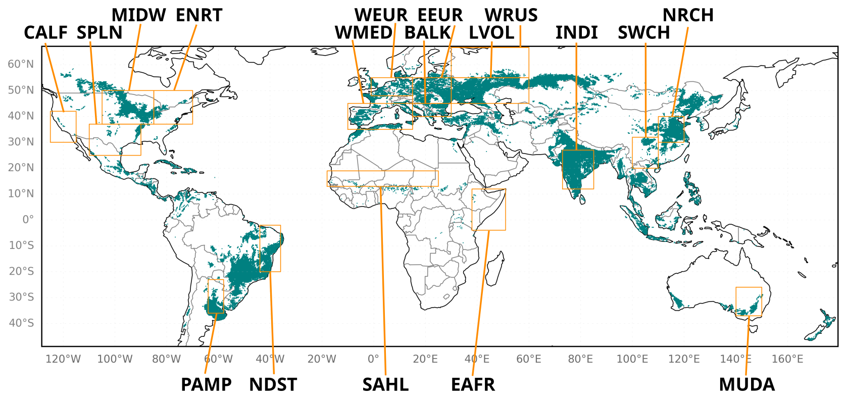
Figure 1 Map of the model domain, where the green areas display the cropland as used in the ISBA model. Orange rectangles denote areas that are especially prone to droughts and heatwaves as identified by Albergel et al. (2020). The regions are named in agreement with the notation of these authors.

As previously mentioned, our focus is on cropland due to the higher sensitivity of microwave observation assimilation found in previous studies. With this restriction, we perform experiments on the global domain with a grid sampling of 0.25°. The selection process is based on the patches extracted from the PGD (Sect. 3.1), whereby only grid cells with a total fraction of C₃ and C₄ crops of 50 % or more are considered (Fig. 1). The terms C₃ and C₄ refer to two different types of carbon fixation in plants, mainly differing by their efficiency of photosynthesis, which depends on their specific photorespiration rate (Slack and Hatch, 1967).

The actual impact of the observations on the analysis is controlled by the ratio between background and observation errors. The background errors are prescribed as 0.2 scaled with the LAI or the dynamic range of the soil moisture, respectively.

As a standard approach, we keep the observation errors of the brightness temperatures constant for all grid points. The initial observation errors for each of the observations are derived from the O–B time series obtained after the training of the NN (see Sect. 4).

4 A neural network as observation operator

4.1 Description of the method

To enable the direct comparison of observations and background required in the assimilation system, the model variables (Sect. 3.1) have to be transformed into observation space. Since the standard approach with a radiative transfer model usually occupies a lot of resources, we develop an observation operator that is based on an artificial neural network.

Our strategy is to train a NN on the T_b observations of each sensor separately in a first step, and to subsequently apply the resulting weights as an observation operator to the model variables during the assimilation cycle (Fig. 2). This strategy was applied before (Shan et al., 2022; Corchia et al., 2023; Shan et al., 2024) on ASCAT observations. In the assimilation cycle, the observations of each sensor are assimilated separately. Training and assimilation of both sensors simultaneously is possible. However, a separate treatment is required at this stage of research to understand the behaviour of the system.

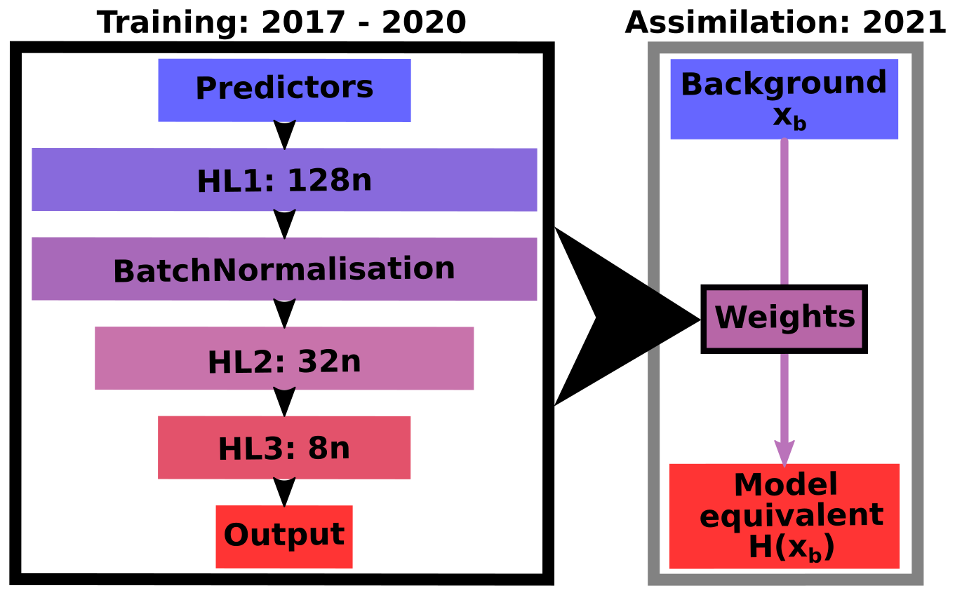
Figure 2 Sketch of the functionality of the observation operator. The architecture of the neural network is characterised by the input (predictors), the output, the hidden layers (HL), and the neurons (n).

To find the best setup, we explore the hyperparameter space of a feedforward NN, that means, different numbers of hidden layers, the number of neurons per layer, and learning rates. Eventually, the training turned out to not be very sensitive to the hyperparameters. This behaviour was already noticed by De Gélis et al. (2025) for the training on snow surfaces. Therefore and in regard of the time consumption of the training, a full brute-force scanning of the parameter space seemed neither necessary nor feasible. Instead, we varied each hyperparameter in several steps, choosing the optimum in terms of evaluated statistics of the obtained model equivalent vs. the observations in the testing period before varying the next hyperparameter.

Our data set spans five years (January 2017–December 2021) and is divided into training, validation, and test data with a fraction of 60 %/20 %/20 %, respectively, where training and validation data are drawn randomly from the same period, whereas the test period covers the subsequent independent time span (2021).

For the input fields, we employ observed LAI (Sect. 2.3) as well as different static (e.g., coordinates, physiographic data) and variable model fields as predictors and analyse their contribution to the final training performance. Since the ISBA LAI is known to be biased (e.g., Albergel et al., 2017), we expect more accurate information from observed LAI.

As model fields, we select soil moisture and temperature of the soil layer (0.01–0.04 m), which corresponds to the second layer in the ISBA model. Deeper layers can be used as well in principle, but tests did not show any benefits, which is likely due to the strong cross-correlation of the different layers, i.e. no additional information is brought into the system. The top most layer (0–0.01 m) is subject to rapid changes determined by atmospheric forcing and therefore, generally considered challenging in the context of assimilation (Draper et al., 2009; Vural et al., 2021). Unlike X-band measurements, such as those taken by AMSR2, which have a shallower penetration depth, observations at longer wavelengths, such as the L-band (SMAP), are more sensitive to the subsurface soil layer (Escorihuela et al., 2010; Entekhabi et al., 2010; Yee et al., 2017).

Passive observations are highly dependent on surface altitude and surface roughness at different scales (Mätzler and Standley, 2000; Njoku and Chan, 2006; Monerris et al., 2008). Consequently, terrain altitude and topographic complexity are expected to be important factors in the accurate simulation of brightness temperatures.

Depending on the wavelength, microwave observations are more or less affected by the atmosphere. Thus, atmospheric effects cannot be completely neglected when retrieving surface variables from microwave emissions, especially at the X band. To account for this, we also examine the effect of using relevant atmospheric forcing variables (see Sect. 3.1) as predictors, such as air temperature and humidity (Tair, Qair), long-wave downwelling radiation (LWdown) and shortwave downwelling direct and scattered radiation (SWdir, SWsca). We are aware that other variables might contribute as well to the brightness temperatures. At one point, too many predictors might increase the probability of overfitting though. As a consequence, we try to keep the number of predictors small and, additionally, test the systematic omission of static predictors.

We trained on brightness temperatures of both H- and V-polarisations originally. In accordance with the findings of Corchia (2024), we found that the addition of H polarisation is not able to improve the skill metrics of the NN significantly compared to training on V-polarisation only (see Appendix A). Training on one output variable only might be a simpler task for the NN in some cases but, here, it can be assumed that the two not independent output variables impose more constraints on the NN, which could theoretically help to improve the results. Output interferences and individual loss behaviour might complicate the training process in cases where the architecture of the NN constrains the training process too much. This is an unlikely scenario in our setup, since we test systematically through multiple combinations of input variables using a multi-layer architecture.

We additionally found that H polarisation yields significantly higher RMSE values than the V polarisation. This is probably due to the generally higher variability of emissivity in the H polarisation (see De Gélis et al., 2025), which seems to be difficult for the NN to match.

Furthermore, Appendix B shows results of employing one of the simplest configuration of predictors (LAI, the soil water index in the soil layer between 0.01–0.04 m (SWI2), and soil temperature in the soil layer between 0.01–0.04 m (TG2)) to demonstrate the need for additional predictors.

4.2 Performance of the neural network

An overview of all tested input parameters together with the bias, the root-mean-square error (RMSE), and the Pearson correlation coefficient is given in Table 1 to evaluate the performance of the model equivalent in comparison with the actual observations. To assess all skill metrics, including as well the standard deviation (SD), at the same time, they are displayed in a Taylor diagram (Taylor, 2001, Fig. 3), where the best experiments are those closest to the observations.

Table 1 Overview of training experiments (exp) for both SMAP and AMSR2 with the predictors that were varied as well as SD (in K), RMSE (in K), correlation coefficient (ρ_P), and bias (in K). The columns describe the longitude (lon), latitude (lat), day of the year (DOY), LAI, soil water index at level 2 (SWI2), soil temperature at level 2 (TG2), altitude (ZS), topographic complexity (ToCo), air temperature (Tair), air humidity (Qair), long-wave radiation (LW), direct short-wave radiation (SWdir), and scattered short-wave radiation (SWsca). The experiments employed later on for data assimilation (Sect. 5) are highlighted with bold font.

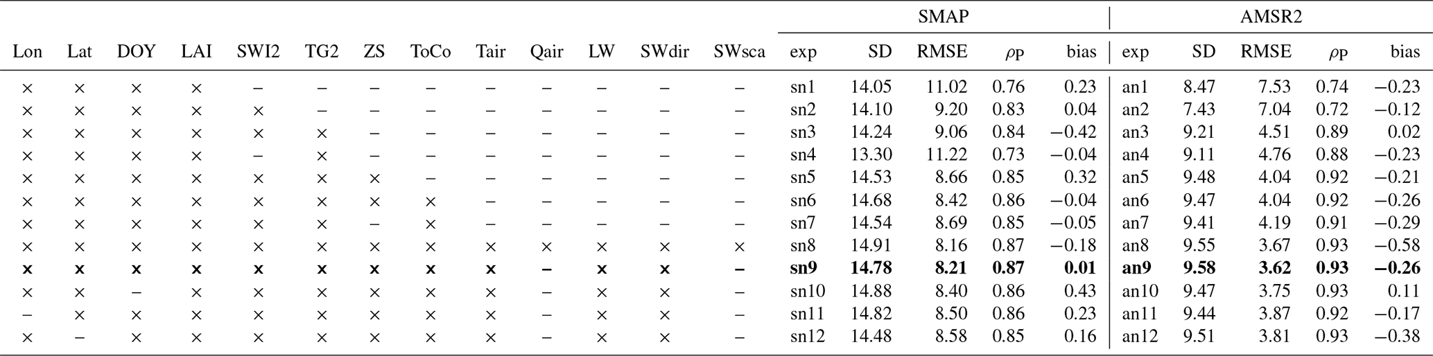
The Taylor diagram and Table 1 suggest that most of the experiments are actually quite similar. There is a clear trend towards better matching of SD, RMSE and correlation, as well as poor performance by experiments that do not use enough surface variables as predictors. Both, Fig. 3 and Table 1 show that biases in both directions can remain. This is an indication that the NN is either lacking information, as in e.g. sn10 and an12, that keeps the simulated data close to the observations on average but also too many predictors as in an8 seem to result in an unbalanced system.

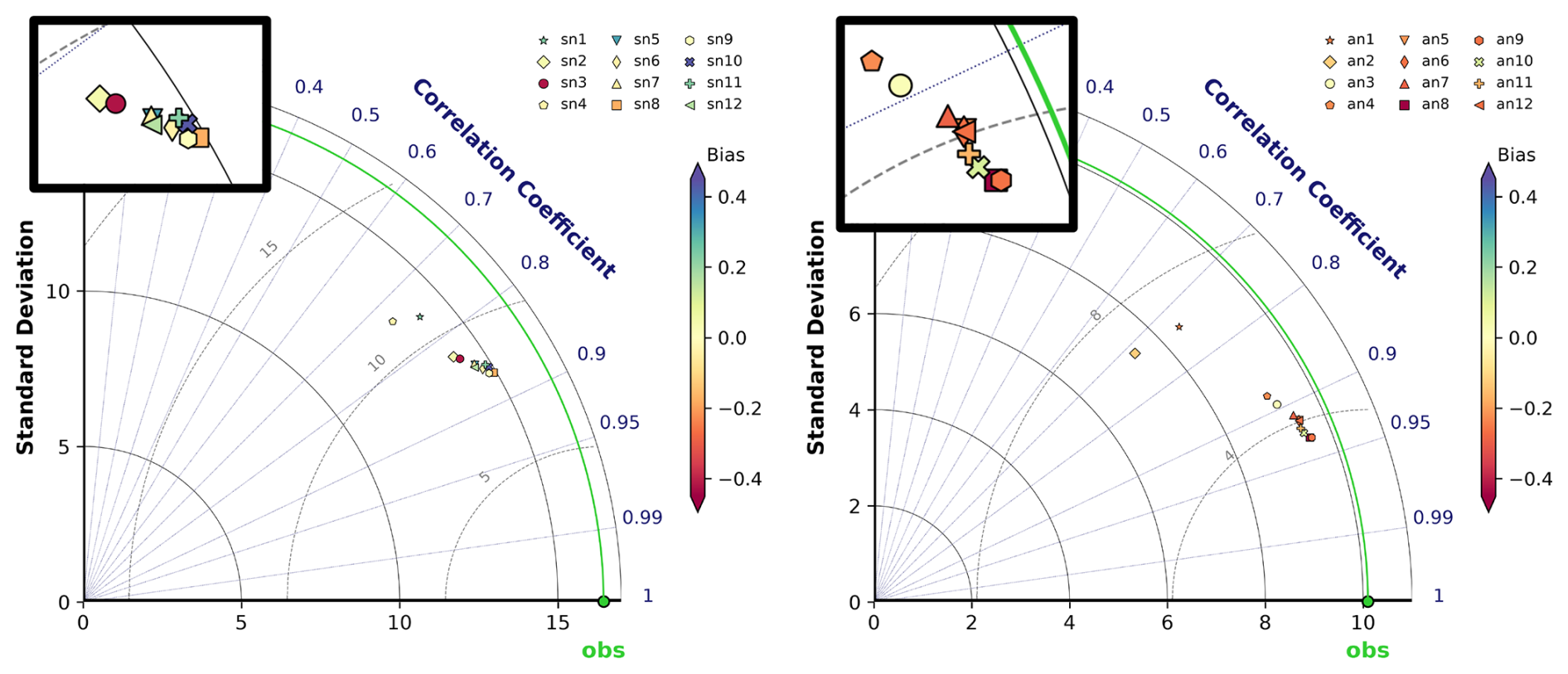
Figure 3 Taylor diagrams (adapted from Rochford, 2016) of SMAP (left) and AMSR (right) training experiments described in Table 1. The SD is shown on the x- and y-axes, the correlation coefficient corresponds to the polar angle, the RMSE is marked by the distance from the observations (green point), and the bias is indicated by the colour of the respective point, zooms on the dense point clouds are inserted within the black rectangles.

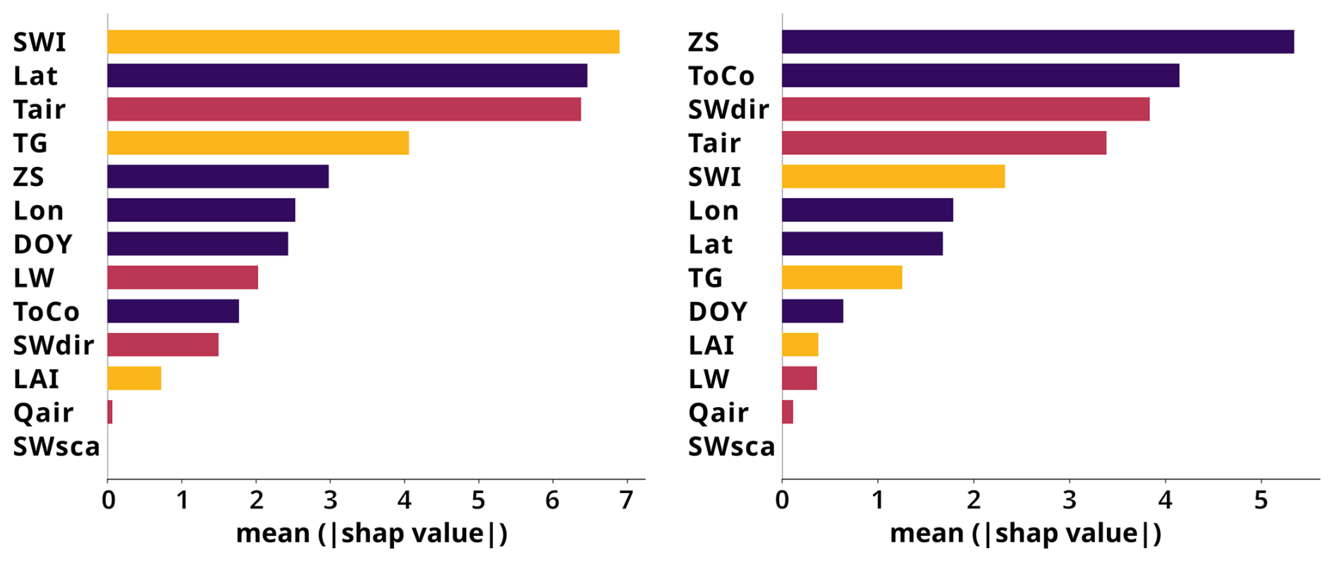
Figure 4 Feature importance using Shapley values of training experiments using all tested predictors for SMAP (left) and AMSR2 (right). Static predictors are indicated in dark violet, forcing variables in red, and surface variables in orange. The displayed variables are the longitude (Lon), latitude (Lat), day of the year (DOY), LAI, soil water index at level 2 (SWI), soil temperature at level 2 (TG), altitude (ZS), topographic complexity (ToCo), air temperature (Tair), air humidity (Qair), long wave radiation (LW), direct short wave radiation (SWdir), and scattered short wave radiation (SWsca).

In addition to the predictors that have already been employed in similar studies, we achieved a significant improvement to the model equivalent by using the variables employed for the atmospheric forcing within LDAS-Monde (cf. Sect. 3.1). As overfitting by using too many predictors has to be avoided, we systematically omit predictors to test for redundancy. In addition, we compute the feature importance based on a measure developed originally in cooperative game theory, so-called Shapley values, using the SHAP library of python (Lundberg and Lee, 2017, Fig. 4). Some static predictors, especially latitude (SMAP) or ZS (altitude, AMSR2), have a high importance but as well SWI2, Tair (near-surface air temperature), and TG2. We suspect that the coordinates, especially latitude, provide information on fine-scale regional patterns that the other predictors do not capture sufficiently.

The LAI seems of minor importance though, which might be due to the NN extracting similar and additional information from other variable combinations, which cannot be further identified here. To verify our approach using observed LAI for the training, we also validated a NN trained on observations against model LAI and compare with a NN using only model LAI for training and verification (Appendix C). We tested this on one configuration for each sensor and, at least for those cases, the results indicate that our approach is stable enough for being used in the assimilation process, where just model LAI is available.

Direct shortwave radiation (SWdir) seems to be exploited very differently by the two instruments. This indicates that AMSR2 brightness temperatures are more sensitive to short-range diurnal variations.

Furthermore, measuring brightness temperatures during the transition phase between day at night like for SMAP, which has overpass times at 6am and 6pm, could make the training more difficult since the state of the atmosphere is changing more rapidly and variations of the variables might be more difficult to learn by the NN compared to a time of the day with more constant solar irradiation. Since we observe that L-band brightness temperatures are more variable than X-band brightness temperatures, we do not assume that this is the dominant effect though.

Some predictors show only a minor feature importance (Fig. 4). We therefore tested whether some of them, especially the static predictors might have become redundant. We found that omitting any of them degraded the performance (Table 1, Fig. 3). We suspect that the strong benefit seen upon adding the forcing variables is primarily due to the inclusion of information of the diurnal cycle that is not present in TG2. This is supported by the fact that omitting one of the variables exhibiting a diurnal cycle slightly degrades the performance again.

This evaluation is based on training on the maximum numbers of predictors employed here and the SHAP library only works with a limited sample of the whole data set. Nevertheless, these findings are mostly consistent among the different experiments and runs.

As expected, adding variables of deeper soil layers did not bring further impact (not shown here) since the observations cannot penetrate deep into the ground.

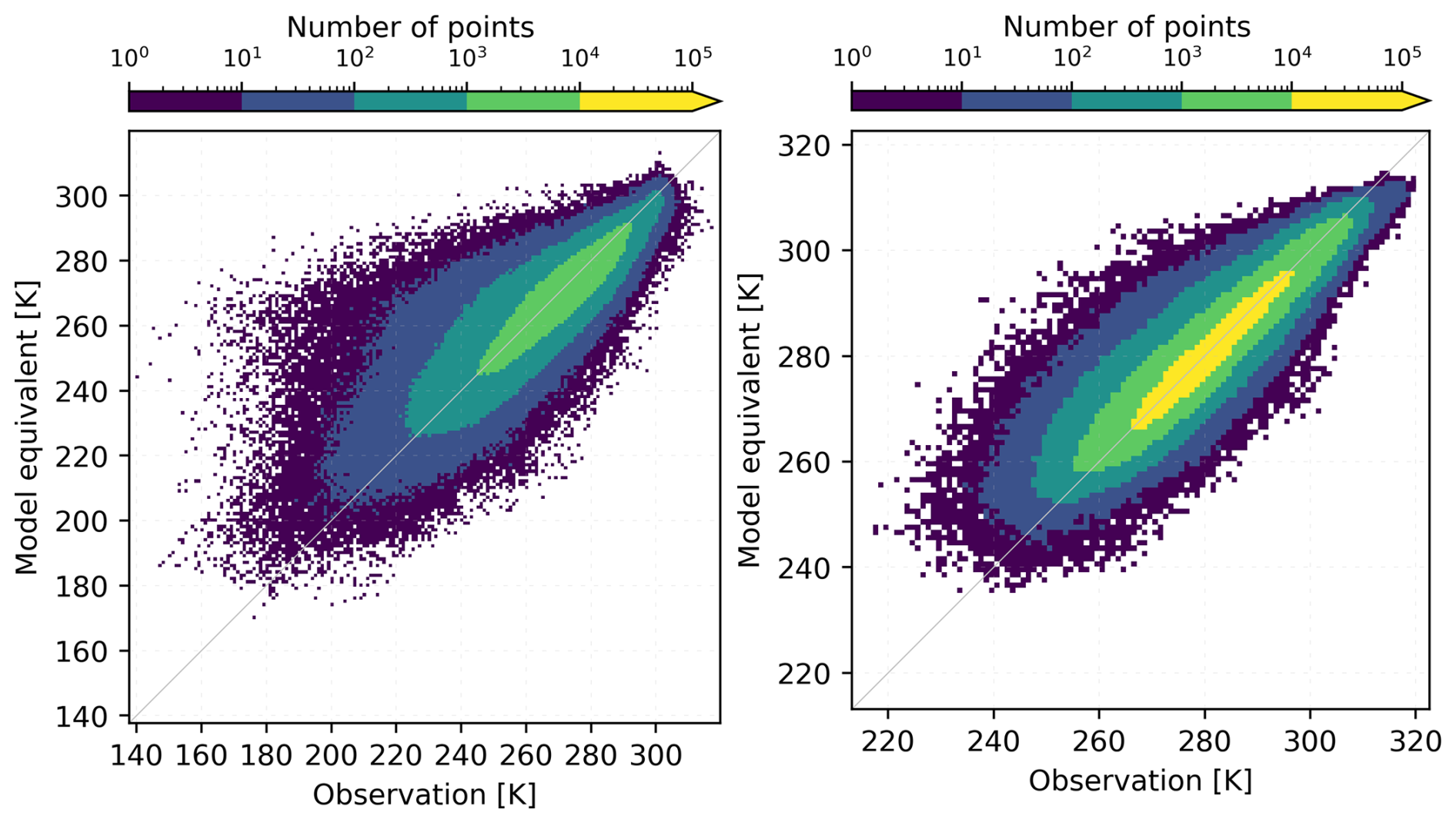
Figure 5 2D histograms comparing model equivalents and observations for SMAP (exp sn9; left) and AMSR2 (exp an9; right).

With respect to all displayed metrics (Table 1, Fig. 3), experiment sn9 for SMAP and experiment an9 for AMSR2 are selected for the following discussion and for assimilation. For the SMAP observations, the 2D-histogram (Fig. 5, left) shows that whereas the vast majority of points is close to the diagonal, a number of especially low-value observations is not matched well. The correlation coefficient reaches 0.87 (Table 1) with better values in the Northern hemisphere but also Australia (Fig. 6, top right). The RMSE is on average around 8.2 K with best values occurring in Europe, Brazil, and Indonesia (Fig. 6, top left).

Figure 6 RMSE (left) and correlation (right) between observations (top: SMAP, bottom: AMSR2) and model equivalent for the best experiments identified in Sect. 4 (exp sn9 and exp an9, respectively, according to Table 1).

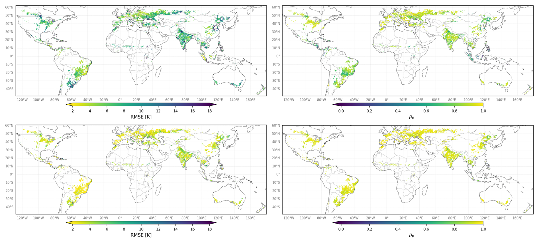
In general, the AMSR2 observations show less variability and are less subject to flagging than the SMAP observations and are, thus, easier to reproduce by the NN. This is reflected in the performance statistics, where higher correlations (Fig. 6, bottom right) and smaller RMSE (Fig. 6, bottom left) are obtained compared to SMAP. The total correlation reaches 0.93 and exhibits high values all around the globe. The spatially averaged RMSE is 3.6 K, with best values in South America and Europe but also in parts of other regions.

The 2D histogram in Fig. 5 (right) for AMSR2 suggests that the negative bias is primarily caused by the tail of the distribution. This means that low values are overestimated, whereas fewer high values are underestimated. The behaviour traced by Fig. 3 indicates that attempting to match the variability of the data more closely is compensated for by an overly strong correction to the mean. In contrast, the SMAP model equivalent (Fig. 5, left) is driven by large scatter at the lower end, which seems to offset the bias for large observation values.

Bad performance often arises from a lack of data during the training period and especially affects areas that exhibit values around the thresholds used for masking, like frozen ground, which occurs mainly in the northernmost latitudes. In these areas, the NN may struggle to describe underrepresented conditions, which could then be simulated using values closer to the temporal average due to the use of static predictors. This could explain a higher RMSE of SMAP in Canada or in the North of Kazakhstan. Areas in China with high RMSE could be the consequence of insufficiently filtered RFI.

Since the penetration depth is larger at L band than at X band, the latter is less sensitive to variations of the soil properties in vegetated areas (Calvet et al., 2011). In return, L band is more affected by agricultural practices. The subsequent larger variability of the L-band signal compared to the X band renders the training process more challenging for the NN, consequently leading to larger errors for the training on SMAP observations.

5 Data assimilation

5.1 Preparation of the assimilation experiments

We implemented the observation operator described in Sect. 4 into our assimilation system (Sect. 3). We would like to recall that the NN was trained with observed LAI to not learn model-inherent biases. In contrast, during assimilation, the derived weights are run on model LAI.

Note that both sensors are treated separately, both during the training phase and during assimilation. In other words, the process flow sketched in Fig. 2 is applied to each sensor individually. While a joint assimilation of both SMAP and AMSR2 observations is technically possible, at this stage of the research we consider the system too immature to progress to the next, more complex stage of joint assimilation.

We ran all assimilation experiments with the same general setup of LDAS-Monde but account for each of the microwave sensors separately, that means that the weights derived by the NN depend on the assimilated instrument with weights from training experiment sn9 for SMAP and training experiment an9 for AMSR2 (cf. Table 1). The assimilation experiments are run over the full year 2021, i.e., the period where the NN was tested and thus no prior knowledge of the observations is contained in the model equivalent.

LDAS-Monde can only run on a 24 h assimilation window, with observations assimilated at a specific time each day. This means that several assimilation cycles must be run to cover the full day if variables with a diurnal cycle are to be fully exploited. To account for this, we ran four separate assimilation cycles at 03:00, 09:00, 15:00, and 21:00 UTC. The assimilated observations were binned into 6 h time bins around these times. This strategy strikes a balance between the time efficiency of the assimilation experiments and the smoothing of the signal over one day due to averaging. Nevertheless, the time constraints only allow for a limited number of assimilation experiments.

5.2 Impact of the observation error

We performed several assimilation experiments for each instrument to investigate the impact of, first, using the forcing variables as predictors and, second, of different magnitudes of observation errors (Table 2). In the following, we adopt the expression “observation error” for “observation error standard deviation”.

Table 2 Overview of the assimilation experiments conducted for SMAP and AMSR2. The table indicates the name of the assimilation experiment (DA exp.), the usage of forcing variables as predictors (forcing), the exact NN experiment as described in Table 1 (NN exp.), and the observation error implemented (obs. err.).

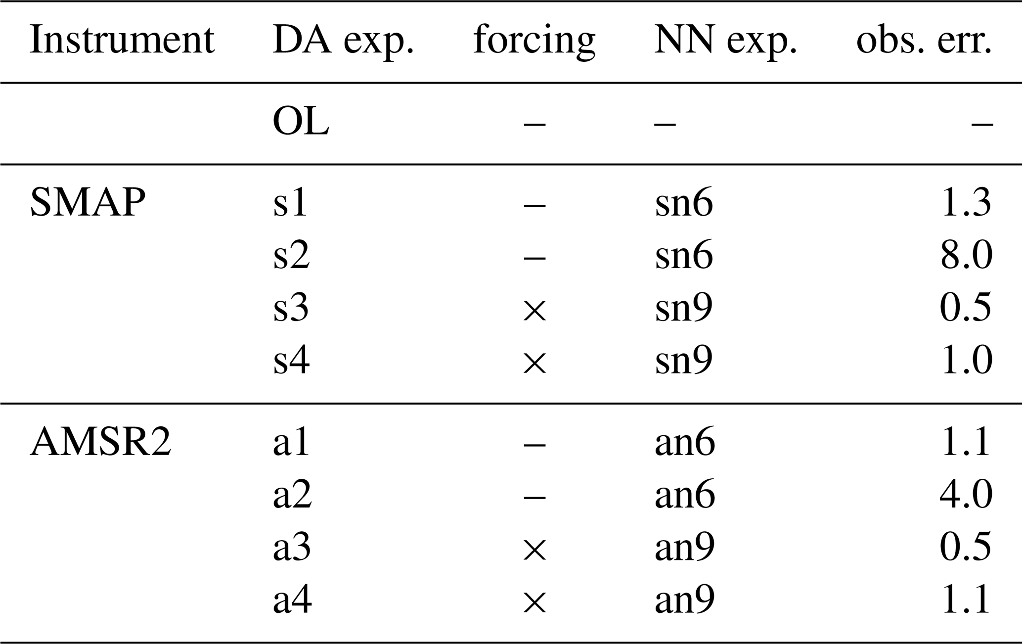
As mentioned in Sect. 3, we derive the initial observation errors σ_o from the O–B time series with 30 % of the average O–B difference, where the background B refers to the OL run here. We compared the errors specified like this in the first experiments (s1, a1 in Table 2) with the errors diagnosed using the method of Desroziers et al. (2005). The larger values were employed subsequently (s2, a2). For the SMOS instrument, which was not investigated here but also operates in L band, Muñoz-Sabater et al. (2018) found that the recommended observation error of 2.5–3 K was too small in a data assimilation context. In contrast, in our assimilation experiments, the error values derived with the help of the Desroziers method (8/4 K for SMAP/AMSR2, respectively) in a first step were too large and diminish the impact of the observations too much, whereas smaller values yield better results. The different behaviour is not only a consequence of the instruments' characteristics but also due to the errors associated to the employed observation operator.

In model space, a range of 0.005–0.015 m³ m⁻³ was found for SMAP soil moisture errors for cropland (Vural et al., 2021) dependent on the grid point and for AMSR2, observation errors in a range of 0–0.38 m³ m⁻³ for China (Fan et al., 2022). These values cannot be compared directly to our findings but indicate that working with one value for the whole domain is not an optimal solution. Since the grid point-wise approach for the estimation of the observation errors is not feasible here, the different constant error values give only a rough estimate. Here, the results show that the larger errors diminish the impact on the analysis too much on a global scale.

The setups including forcing variables as predictors yield smaller initial observation errors using the described approach of a fraction of the average O–B difference, and, of all tested values, we found the errors around 0.5 K most suitable according to the impact on the assimilation system (Sect. 5.3) as well as on the verification (Sect. 5.4). Note that we did not use the diagnosed Desroziers errors here since a similar behaviour as found for s2/a2 can be expected. Indeed, the results indicate that the larger observation errors employed in the s4/a4 experiments have, on average, a slightly smaller positive impact on the analysis than for s3/a3.

We underline that the employed observation errors are empirically-tuned effective observation errors, eventually. The large differences between the diagnosed observation errors and our final values might be a result of unfulfilled conditions. Since uncorrelated background and observation errors are required, it is likely that the part of the observation error that is due to the observation operator is one of the main responsible sources of that deviation. The use of model variables as predictors introduces inter-dependencies here, which cannot be resolved easily.

5.3 Departure statistics

To validate the assimilation of the introduced observations and the behaviour of the developed observation operator, we compare background and analysis departures ($d_{\mathrm{b}}^{\mathrm{o}}$ and $d_{\mathrm{a}}^{\mathrm{o}}$, respectively) of the respective experiment with each other. The system behaves as expected when the assimilation is able to bring the analysis departures closer to zero on average than the background departures. We confirm that this can be considered the case for AMSR2 (Fig. 7, left, for s3 and a3), whereas the mean value of the distribution is drawn slightly to the negative for the SMAP experiment. The distribution of the departures is in general wider for SMAP than for AMSR2, which reflects the behaviour seen already in the evaluation of the NN in the testing period (Sect. 4) and was attributed to the larger variability of the L-band signal compared to the X band as well as the lower number of points remaining for the training after quality control. As a consequence, the assimilation is able to yield a larger change for SMAP, whereby the distribution appears to be generally more confined to zero but slightly shifted to the negative (difference of mean $\mathrm{\Delta }\mathit{\mu }\approx -\mathrm{0.27}$ K, difference of SD Δσ≈0.54 K). The change for AMSR2 is less pronounced (Δμ≈0.08 K, Δσ≈0.24 K) since the model equivalent is already quite close to the observations.

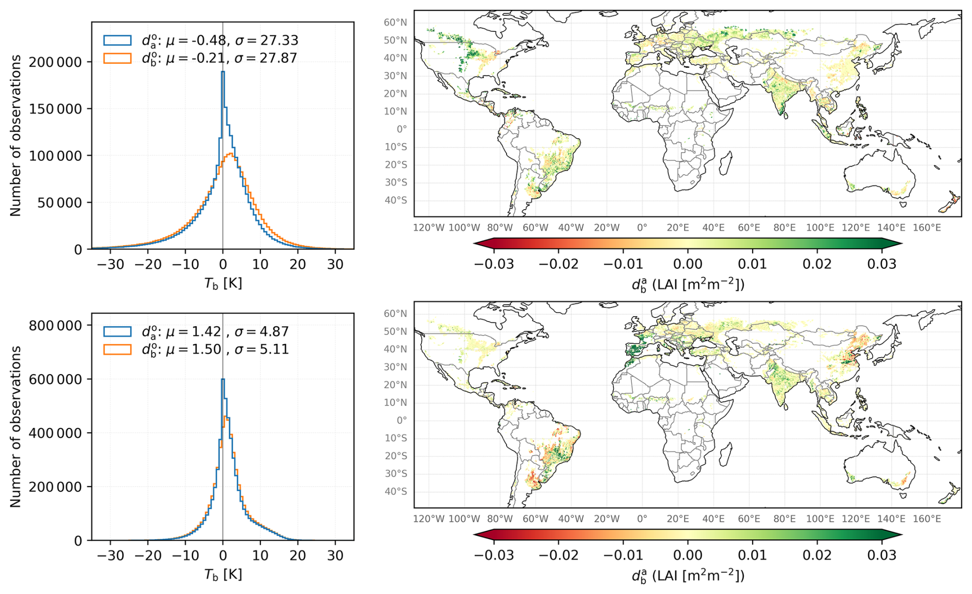
Figure 7 Left: Histograms of innovations ($d_{\mathrm{b}}^{\mathrm{o}}$, orange) and residuals ($d_{\mathrm{a}}^{\mathrm{o}}$, blue) for experiment s3 (top) and a3 (bottom). Right: Distribution of accumulated increments $d_{\mathrm{b}}^{\mathrm{a}}$ for experiments s3 (top) and a3 (bottom).

The LAI increments range between −1 and 1 due to constraints in the assimilation system with a pronounced maximum around zero indicating as many positive as negative increments. Nevertheless, the spatial distribution (Fig. 7, right) shows that some areas are impacted more by the assimilation on average, namely Southwest Russia, Northern US, and Canada, where LAI is mostly added by the SMAP observations. In contrast, the AMSR2 observations remove LAI dominantly in Southern America and adds LAI in Western Europe, whereas Northeast China is marked by strong increments of both signs.

Soil moisture increments are on average rather small. They decrease more than increase for both instruments for the second and third soil layers, with more symmetric distributions in the deeper layers (not shown here). Apparently, not all removed soil water is distributed to the LAI but might also be subject to increased evaporation.

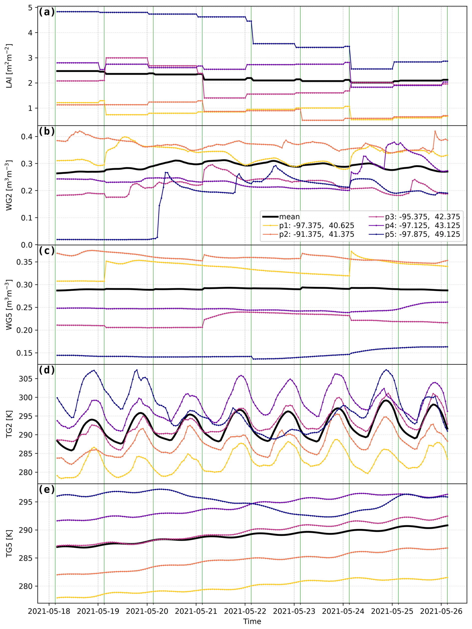
Figure 8 Model evolution in the region MIDW between 18 and 26 May 2021. The panels show the LAI (a), surface and root zone soil moisture (WG2: b, WG5: c), as well as surface and root zone temperature (TG2: d, TG5: e) for five different selected grid points p1–p5 (coloured lines) with coordinates indicated in the legend and the average over the whole region (black line). The green lines indicate the assimilation time 03:00 UTC, the LAI is computed at 00:00 UTC. For clarity, the curves for the single grid points of TG2 and TG5 are offset by 5 K from each other.

To study the impact of the analysis on the model evolution in detail, we select one of the regions described in Sect. 3.2 (MIDW here) and monitor the time series for LAI as well as for both surface and root-zone (0.4–0.6 m) soil moisture (WG2, WG5) and temperature (TG2, TG5) for experiment s3 with the assimilation time at 03:00 UTC. We select five grid points where the impact of the increment on the control variables is visible clearly (Fig. 8).

The LAI is computed once per day at 00:00 UTC, thus the updated values persist throughout the day. There are cases, where the subsequent model step corrects to the opposite direction of the previously added increment. This can be considered as regular behaviour since the time in between allows for evolution of other variables. WG2 shows that the simulation seems consistent even in those cases, e.g. p3 on 24/25 May 2021.

The strength of the impact on LAI and WG2 does not always correlate, e.g., point p2 at 21 May 2021 receives a large negative increment for LAI but WG2 seems not impacted. In contrast, large LAI increments can be correlated with larger opposite increments in WG5 (e.g., p1 on 19/24 May 2021).

We also see the impact of a rain event on WG2 of p5, which is not taken into account by the LAI since it is developing on longer time scales. In the root zone, increments can be both smaller or larger than in the surface layer. In general, the model seems to evolve naturally after the analysis step. For temperature, which is not in the control vector, no direct impact of the analysis is visible. This indicates that the temperature evolution is not strongly coupled to soil moisture and LAI on a daily basis. Rain events can be partially traced in TG2 by a decrease in temperature, whereas TG5 naturally features a smooth development. Especially TG2 is dominated by the hourly atmospheric forcing. Nevertheless, TG2 and its errors can influence the increments due to its impact onto the observation operator (Fig. 4).

The figure shows that increments introduce small changes on average, which can be followed by the model evolution. For LAI, the assimilation seems to counteract the natural model dynamics. This behaviour is most likely due to the model not accounting for agricultural practices, which can be captured in return by observations.

Obviously, these results cannot be generalised, however, they give an impression of how the assimilation system works.

5.4 Verification against LAI observations

For verifying the impact of the assimilation, the analyses are compared against an independent observational data set for LAI (CGLS; Sect. 2.3) to evaluate a potential improvement compared to the OL run.

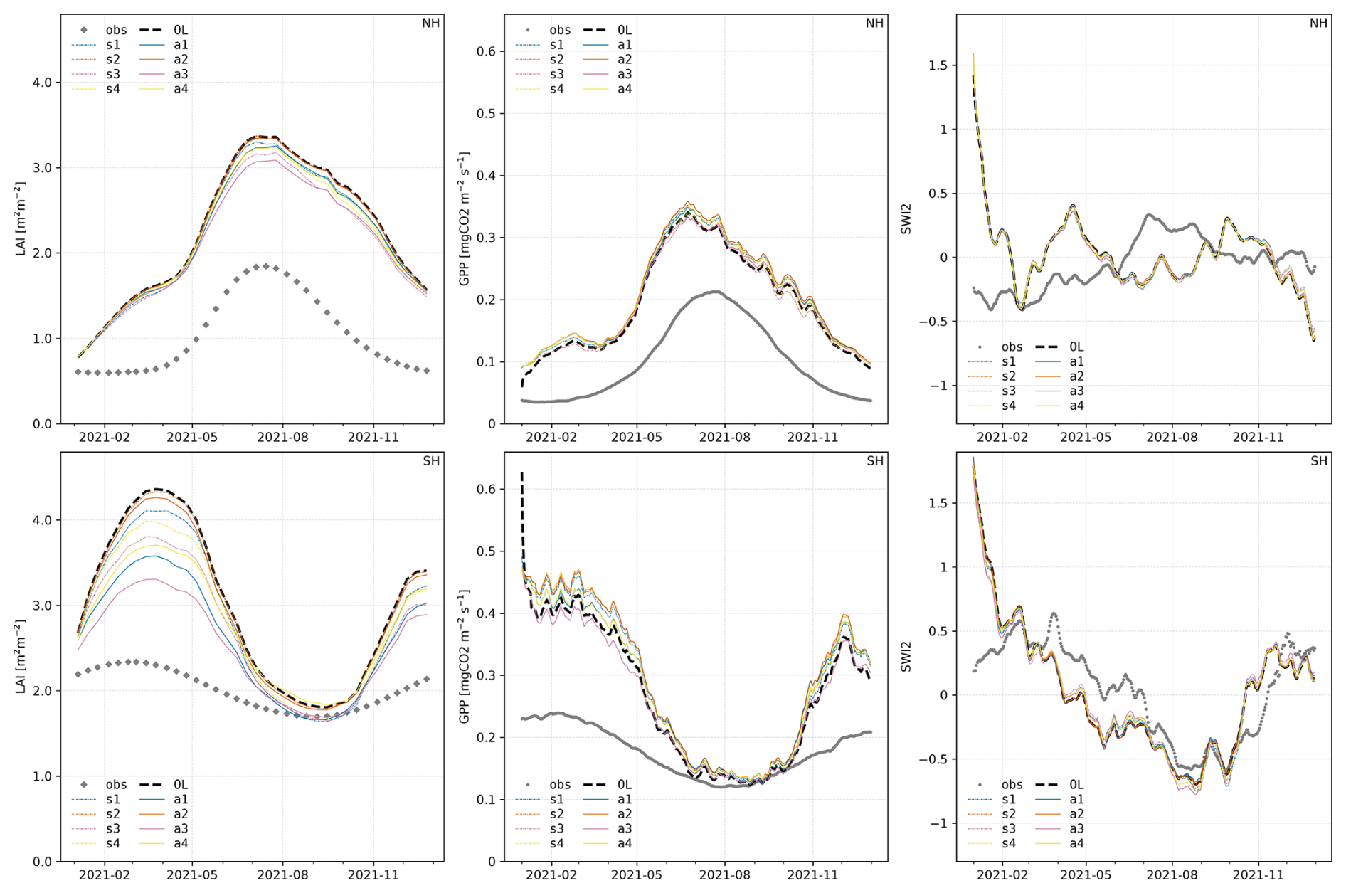
Figure 9 Comparison of time series of LAI (left), GPP (centre), and scaled SWI anomalies (right) averaged over global cropland for northern (NH; top row) and southern hemisphere (SH; bottom row). Observations (gray points), OL (black dashed line), and DA experiments (SMAP: dash-dotted lines, AMSR2: solid lines) are shown in comparison. For clarity, we smoothed the lines of GPP and SWI anomalies by applying a 10 d rolling average.

To account for the different seasonal cycles, we divided the dataset into northern (NH) and southern (SH) hemispheres when evaluating the temporal evolution. For both the SMAP and AMSR2 instruments, we obtained an improvement of the temporal evolution of the LAI compared to the OL run for almost all experiments on both the NH and the SH (Fig. 9), with a more pronounced impact on the latter. In general, the LAI analyses do not match the temporal evolution of the observations very well. This effect is mostly achieved by an improvement in bias as also noted by Albergel et al. (2020), both unbiased RMSE (ubRMSE) and correlation are not improved in most cases (cf. Fig. 10). Nevertheless, all experiments except s1 and s2 are able to improve the RMSE in most of the investigated regions compared to the OL (Fig. 10).

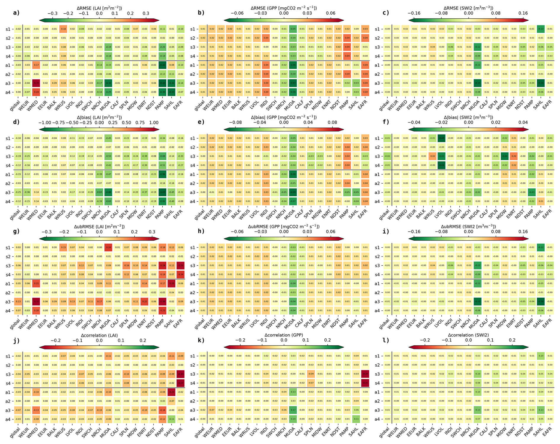
Figure 10 Score cards displaying the difference of RMSE (a–c), absolute bias (d–f), ubRMSE (g–i) and correlation (j–l) compared to the OL for LAI (a, d, g), GPP (b, e, h), and SWI2 anomaly (c, f, i). The metrics are computed between analysis/OL and observations for all investigated assimilation experiments (Table 2) for each of the regions prone to droughts (Albergel et al., 2020, Fig. 1). Green colours indicate an improvement compared to the OL, red a degradation. The boxes are labelled with the respective values.

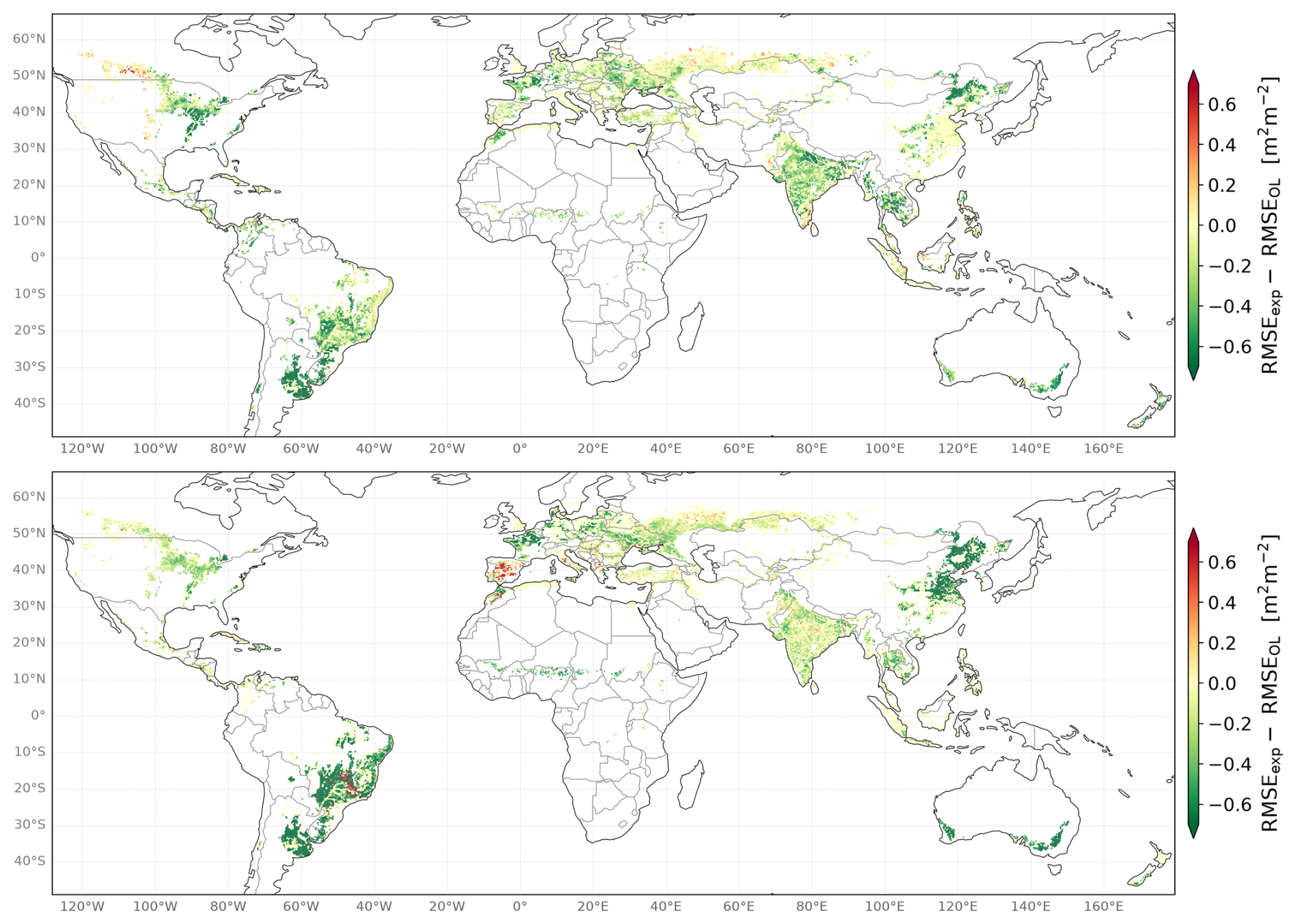
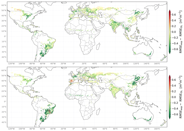
Figure 11 Verification against observed LAI. Difference between the RMSE of the LAI of the DA experiment and the OL for experiments s3 (top) and a3 (bottom) over the whole assimilation period (2021).

For experiment a3, the aggregated RMSE maps (Fig. 11, bottom) show a strong relative improvement over Australia, East Asia, and parts of South America, but a degradation of parts of Western Europe and Brazil. The rest of the globe exhibits a smaller mixed impact with a more negative impact in Ukraine and West Russia.

The spatial distribution for experiment s3 shows as well an improvement in Australia, in East Asia and Brazil as well as in India but a scattered degradation at high latitudes, especially in Canada. For the rest of the globe, we obtain mostly a mixed to positive impact, albeit with less amplitude than for a3.

Furthermore, we investigated the impact of the assimilation on specific areas especially affected by droughts and heat waves as identified by Albergel et al. (2020, Fig. 1) since detailed knowledge about the ambient conditions is crucial for disaster management.

As for the global time series, the temporal match for the different regions is determined by the OL bias and, thus, not very pronounced in the analyses. With regard to the overall improvement of the RMSE, the score card (Fig. 10a) illustrates the challenge to find one experiment that is suited to improve on all investigated areas. Whereas India (INDI), Northern China (NRCH), the Murray-Darling basin (MUDA), the Pampas (PAMP), and East Africa (EAFR) are better represented by all experiments, the representation of the LAI in West Russia (WRUS) seems to be difficult to improve by the employed observations independently of the experiment. This is in agreement with the lower performance seen in that area on spatial scale (Fig. 11).

Figure 10d, g illustrate that the RMSE improvements are mostly driven by improvements in the bias, which are obtained for almost all cases, whereas the ubRMSE is degraded mostly. The correlation is degraded almost everywhere (Fig. 10j).

Eventually, the shown evaluation is mostly in favour for the implementation of a predictor set making use of forcing variables, underlining the necessity to include more information on the diurnal cycle within the training process. The assessment of the observation errors remains a challenge, nevertheless, our assimilation experiments show that large errors dilute the impact of the observations onto the analysis too much (s2 and a2 in Fig. 10).

5.5 Verification against GPP observations

Similar to Sect. 5.4, we verified the impact of the analyses against the GPP FLUXCOM-X (Sect. 2.4).

As for LAI, the impact on GPP is more pronounced on the SH than for the NH (Fig. 9). The experiments do not differ greatly from each other in the NH, and in most of the experiments in both hemispheres, the assimilation moves the analyses further away from GPP observations. The extreme mismatch in the time series of the OL run is seemingly hard to correct. The strongest positive impact is seen for a3 in the SH, however, the initial improvement cannot be maintained over southern winter where the sensitivity of vegetation-driven processes is naturally lower.

Nevertheless, a positive impact on the RMSE can be observed for several regions, especially for NRCH and MUDA, but also for SWCH and CALF, for a3 and a4 additionally PAMP and SAHL, for s3 and s4 additionally SPLN and MIDW, and EAFR (Fig. 11). These areas are mostly those where a strong positive impact was noticed already in the RMSE of the LAI. Furthermore, as for LAI, a large part of the impact results from an improvement in bias (Fig. 10e). A slight improvement in ubRMSE is obtained though for mainly the NRCH, MUDA, and CALF regions (Fig. 10h). The impact on the correlation is mostly neutral with a strong degradation of s3 and s4 in EAFR and an improvement for few experiments in the MUDA and SAHL regions (Fig. 10k).

5.6 Verification against SWI observations

Measured soil moisture and, hence, SWI cannot be compared accurately to model values due to the inherent representivity mismatch. As a consequence, we compute SWI anomalies (cf. Sect. 2.5) for the soil layer between 0.01–0.04 m and compare those.

The impact on SWI anomalies is mostly negligible in the NH (Fig. 9, top right). In the SH, several experiments slightly improve the SWI compared to the OL but not consistently over the whole year.

The impact on the single regions is neutral to positive in total with the largest improvements for MUDA and SAHL (Fig. 10c). Here, the changes in RMSE do not seem to be induced by the change in bias (Fig. 10f). The impact on correlation is neutral for most regions with a tendency to a positive impact for especially MUDA and SAHL (Fig. 10i).

AMSR2 experiments tend to yield a slightly larger improvement than the SMAP experiments. Since L-band observations are generally more sensitive to soil moisture than X-band observations, this seems unexpected. Considering the variability characteristics of the brightness temperatures, this could be another implication of the smoother AMSR2 signal being easier to reproduce by the observation operator and, eventually, being able to introduce more suitable increments.

We cannot exclude that the observation operator may have neglected physical connections, resulting in unrealistic increments being added to the model background in some places. As exemplarily depicted in Sect. 5.3 on a selected area for a short time range, the model evolution does not show obvious inconsistencies. Given the limited scope of this investigation, these findings cannot be generalised necessarily.

6 Discussion

Section 4 showed that an observation operator can be constructed in a rather simple fashion. Improvements could still be achieved by, e.g., combing different architectures of the NN with the different predictor sets or exploring other data sources. Nevertheless, our study showed that a good agreement between the model equivalent created by the NN and the observations can be achieved with a simple architecture. Eventually, the goal of an observation operator is not to perfectly match the observations as no correction would be achieved by data assimilation in that case.

In Sect. 4.2, we demonstrated that static predictors are essential for our data sets, even more for AMSR2 than for SMAP (Fig. 4). As mentioned, static predictors may help to classify information obtained from variable predictors more effectively depending on the exact location. It would, however, be interesting to find a configuration with less need to train on information from static predictors to potentially overcome issues at the edges of the distribution. Other studies showed that the approach of a coordinate-independent NN for each grid point is able to achieve reasonable results as well on a small scale (Shan et al., 2022; Corchia et al., 2023).

The small biases found for the model equivalent (Sect. 4, Table 1) justified the assimilation without bias correction of the observations. Nevertheless, the main benefit in model space after assimilation seems the improvement of bias for the LAI as was shown in Sect. 5.4. This impacts the RMSE positively, whereas correlation and ubRMSE do not profit from the assimilation.

This behaviour can partially be attributed to our model run: Since the OL is subject to a large mismatch, which is likely due to a bias in the forcing data, it is consequently difficult for the assimilated observations to fully correct for this.

For both main experiments s3 and a3 for SMAP and AMSR2, respectively, a degradation for high latitudes was noticed. This seems similar to the findings of Corchia (2024) for the assimilation of both ASCAT and SMOS observations. This degradation might be related to the sensitivity of the observations to frozen soil and, possibly, the subsequent lack of training data in case the masking does not affect the whole of the period.

Eventually, the onset of vegetation growth is often not well captured by the model and a lack of it in the beginning of the season is challenging to correct by the observations. Biases introduced by ERA5 forcing were already investigated (e.g., Calvet et al., 2020; Liu et al., 2025) and are generally attributed to systematic errors in the cloud detection (Urraca et al., 2018). Furthermore, brightness temperatures are sensitive to the representation of soil temperature in the ISBA model and soil temperature biases (Calvet et al., 2020; Verger et al., 2025; Rojas-Munoz et al., 2026).

The separate investigation of areas prone to droughts showed that both sensors have their strengths in different areas. This is expected as the different microwave bands have different characteristics. In terms of RMSE and bias, the assimilation often yields a better match with the LAI observation than the OL, especially AMSR2 is able to achieve a large improvement. On the other hand, large positive increments (Fig. 7) can also lead to stronger degradations as seen in the Mediterranean (WMED). Since the model equivalents (Fig. 2) do not exhibit any characteristics that could explain this behaviour, we suspect that the added LAI at the beginning of the year leads to increased soil water depletion and, consequently, an overestimation of the decrease in LAI during the dry season. As stated before, we cannot exclude that physical connections between the variables are not properly mapped by the observation operator.

This might be as well the cause for the globally minor impact of the assimilation onto the GPP and the SWI anomalies and for the sometimes even opposite effect in correlation. A small impact of the assimilation of an LAI-proxy (vegetation optical depth) retrieved from SMAP and different microwave sensors including AMSR2 on SWI was already found by Kumar et al. (2020).

In general, we can assume that the NN-based observation operator is able to act on one or few variables but since no physics-based optimisation was applied, the model equivalent can seem adequate but still interfere within the assimilation process. This can be due to the possible neglect of inter-variable cross-correlations, which makes the information that is spread onto other variables inconsistent (Shan et al., 2024).

7 Conclusions

In this study, we investigated the advantages of using a neural network as an observation operator in LDAS-Monde for assimilating vertically polarised microwave brightness temperatures. The optimal NN configurations were determined for SMAP L-band and AMSR2 X-band observations using static predictors, LAI observations, as well as forcing and model variables. The setup of the hyperparameters turned out to be of minor importance, whereas a proper pre-processing of the data sets seems essential. In the end, most training experiments were able to reproduce the observations to a satisfactory degree with high correlations of up to 0.87 for SMAP and up to 0.93 for AMSR2.

The total RMSE of 8.2 K for SMAP exceeds the RMSE of 3.6 K for AMSR2. For this, we identified the following reasons: First, the generally lower variability of the X-band brightness temperatures compared to the L band due to their different sensitivities to canopy and soil surface and, second, the much larger amount of data remaining for AMSR2 after quality control, which can feed the NN with more values on the edges of the distributions. With regard to the employed predictors, surface variables seem more important for SMAP, whereas topography and forcing variables play a larger role for AMSR2.

The found performances of the NNs are suitable to produce a model equivalent for both instruments, leading to the subsequent implementation into our assimilation system LDAS-Monde, where the application of the found weights to the model background acts as the actual observation operator.

The assimilation experiments yielded the expected improvement of the residuals compared to the innovations. The improvement is larger for the SMAP than for AMSR2 data, which is likely a consequence of the better match between model equivalent and observations for AMSR2, giving less room for improvement.

When comparing the analyses against independent LAI observations, we obtain an improvement on global scale with generally stronger improvements for NN configurations using forcing variables as predictors and employing smaller observation errors.

Compared to the SMAP assimilation experiments, the AMSR2 experiments better match the temporal evolution of LAI on a global scale, whereas on a spatial scale, SMAP is able to outperform AMSR2 in dependence on the region. With regard to this behaviour, we studied areas especially prone to droughts and identified several regions that benefit strongly from the assimilation, mainly through a reduction in the bias. In contrast to the general trend, SMAP can outperform AMSR2 in some of those regions when considering total metrics. For example, in INDI and ENRT, SMAP has a lower RMSE of LAI and a higher SWI anomaly correlation in MUDA. The verification against GPP and SWI anomaly yields a smaller and sometimes opposite effect on the performance though.

Overall, the results show the potential of assimilating brightness temperatures with a neural network to improve the state estimate of LSVs. Further tuning of the DA system might be required to achieve a more accurate match of the LAI observations, including the solution of model-inherent difficulties with the proper representation of land-surface processes. Eventually, a physics-based training might be able to overcome the observed inconsistencies between different LSVs.

Appendix A: Training of the Neural Network on both H and V polarisation

To address the discussion about the implementation of the H-polarisation brightness temperatures in the training of the NN, we show all experiments in comparison in Fig. A1. The experiments described in Table 1 remain unchanged for both H+V and V-only setups. Slight shifts for single experiments can be spotted but the difference between H+V and V-only setups can be considered negligible for both sensors.

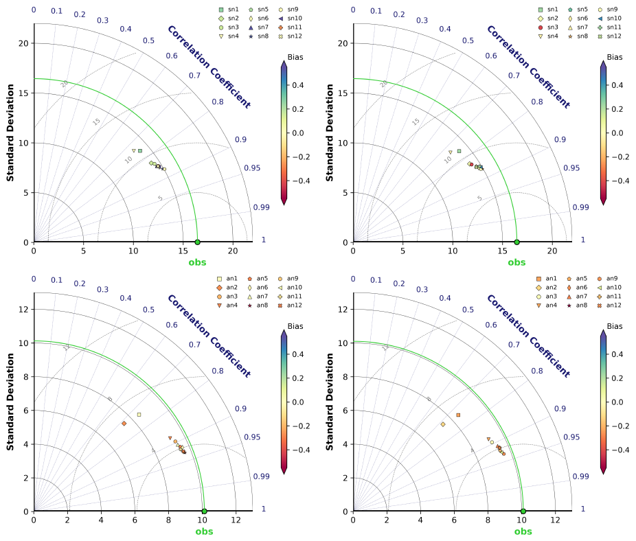
Figure A1 Taylor diagrams of SMAP (top) and AMSR2 (bottom) training experiments (Table 1) comparing training on V polarisation compared to training on H and V polarisation simultaneously. Left: V polarisation trained on H+V. Right: V polarisation trained on V-only. The SD is shown on the x- and y-axes, the correlation coefficient corresponds to the polar angle, the RMSE is marked by the distance from the observations (green point), and the bias is indicated by the colour of the respective point.

Appendix B: Training of the Neural Network without forcing variables or static predictors

To demonstrate the need for additional predictors, we show a training experiment with the very basic predictors only: LAI, SWI2, and TG2. The 2D-histogram (Fig. B1) exhibits a much larger tail for low observation values compared to the best setup shown in Fig. 5 in the main document, a generally larger deviation from the diagonal, and a cap at lower values of the model equivalent.

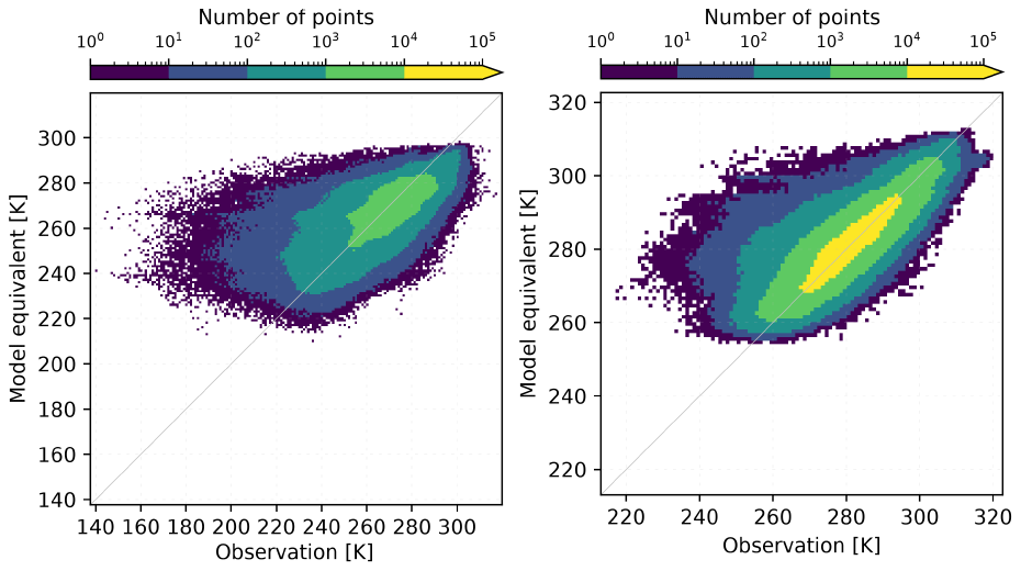
Figure B1 2D histograms comparing model equivalents of an NN using only three predictors and observations for SMAP (left) and AMSR2 (right).

Appendix C: Discussion on using model or observed LAI within the Neural Network

To give an impression on the model bias with respect to LAI observations, Fig. C1 illustrates the systematic overestimation by the model for the time period employed in this study. In the investigated period, we find a bias of −0.73 m² m⁻² over global cropland.

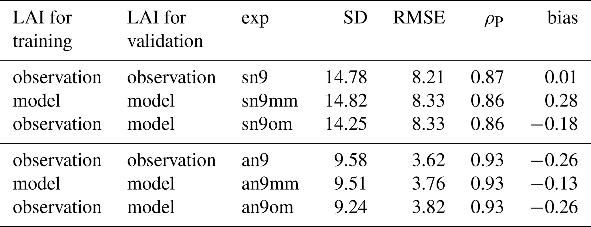
To confirm the validity of the derived relationship for model LAI, we compare the results of one experiment per sensor (sn9/an9) with two additional experiments each (Table C1): one where we validate the NN trained with observed LAI on model LAI (sn9om/an9om) and one where we train and validate with model LAI only (sn9mm/an9mm). Obviously, the results are not identical, the correlation remains about the same though. The bias for an9om shows similar values as an9, whereas the RMSE and SD are slightly more off (SD ≈ 15/10 K for SMAP/AMSR2 observations, respectively). The slightly smaller SD of sn9om/an9om should have a negligible impact on the residuals though (Sect. 5.3). The smaller bias for an9mm seems natural since model simulations are generally smoother and easier to fit than observations.

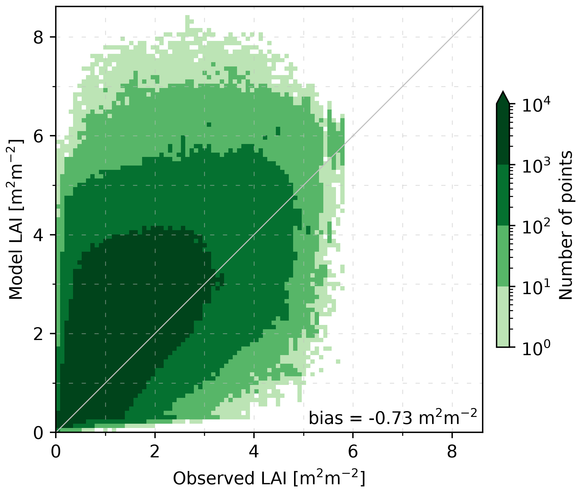
Figure C1 2D histogram comparing model LAI (OL) and LAI observations using the available data between 2017 and 2021 (inclusively) over global cropland. The bias (observation-model) is indicated in the figure.

Table C1 Additional training experiments (exp) for SMAP (sn) and AMSR2 (an) with the SD of the model equivalent (in K), RMSE (in K), correlation coefficient (ρ_P), and the bias (in K). Observation and model refer to the input employed in the NN (Sect. 4).